AN245 - Calibration of the MA600A

In side-shaft configurations, on the other hand, the majority of the magnetic error arises due to the unequal amplitude between the radial and tangential components of the magnetic field across a full rotation. This error can be compensated using a single correction parameter in the MA600A known as bias current trimming (BCT). However, even after this compensation, residual magnetic errors usually persist due to factors such as magnet imperfections or misalignments in sensor or magnet positioning. To obtain a high-accuracy sensor with errors near or below 0.1°, all these remaining deviations must be suppressed. Intrinsic sensor errors and magnetic errors can be effectively corrected through a calibration process storing 32 correction points in the MA600A’s internal memory.

CALIBRATION MECHANISM

Overview

Calibration data is stored in 32 non-volatile memory (NVM) registers, each holding an 8-bit correction value. These values correspond to 32 raw angular positions evenly spaced across a full 360° rotation —specifically, every 11.25°. For angles between these fixed points, the sensor applies linear interpolation to compute the correction.

Memory Mapping of Correction Values

The correction values occupy 32 consecutive 8-bit registers within the MA600A memory, specifically designated as “Block 1.” These span from register 32 (address 0x20) to register 63 (address 0x3F) (see Table 1).

Table 1: Content of the 32 Registers Forming “Block 1” of the Memory

		Registers of Block 1
Index	Lookup Angles	Address		Lookup Correction
I	\[\text{a}_{\text{i}}\]			CORRi(7:0)
	Degree	Decimal	Hex
0	0	32	0x20	CORR0
1	11.25	33	0x21	CORR1
…	…	…	…	…
31	337.5	62	0x3E	CORR30
32	348.75	63	0x3F	CORR31

Each correction value, denoted as CORRi (where i ranges from 0 to 31), is associated with a lookup angle (a_i) corresponding to the uncorrected or “raw” angle for which the lookup correction is given. Although the MA600A outputs angles using a 16-bit word, the correction is applied only to the 8 bits in the middle, resulting in a correction resolution of 12 bits (approximately 0.087° per step) (see Table 2). The 4 LSBs are discarded to optimize memory usage, as they typically fall below the sensor’s repeatability threshold.

To further save memory, the correction range is constrained to ±11.25°. Consequently, the calibration table cannot compensate for errors exceeding this range.

Table 2: Correspondence between the 16-Bit Angle Output and the 8-Bit Correction Stored in the Memory

Bit	15	14	13	12	11	10	9	8	7	6	5	4	3	2	1	0
	MSB				CORRi(7:0)											LSB

The lookup correction values CORRi(7:0) are represented by 8-bit signed integers (in a standard two-complement representation, which is also known as “int8”). To convert these values into the 16-bit resolution corrections terms (corr_i in degrees), the following rules apply.

If the MSB of CORRi(7:0) is 0 (i.e. CORRi(7) = 0), then corr_i is positive, as calculated with Equation (1):

If the MSB of CORRi(7:0) is 1 (i.e. CORRi(7) = 1), then corr_i is negative and must be interpreted using two’s complement, as estimated with Equation (2):

Sensor Operation

During operation, the sensor continuously computes a correction value to adjust the raw angle measurement. This angle measurement is denoted as α. If α falls between the lookup angles a_i and a_i+1, this correction is determined through linear interpolation between two adjacent lookup corrections: corr_i and corr_i+1. corr(α) can be calculated with Equation (3):

Figure 1 shows the linear interpolation between two adjacent lookup correction terms.

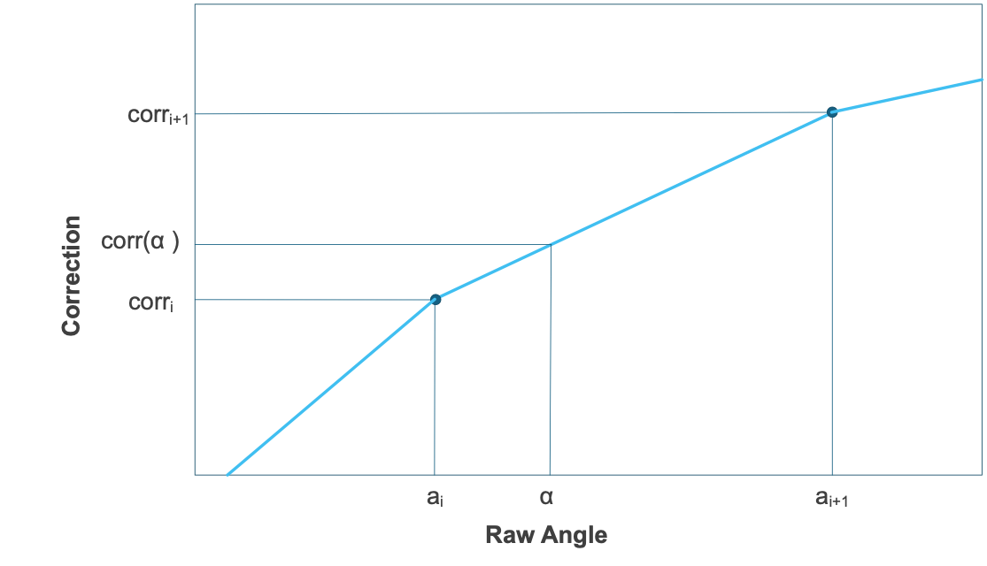
Figure 1: Linear Interpolation between Two Adjacent Lookup Correction Terms

The sensor’s final corrected angle output can be estimated with Equation (4):

It’s important to note that the lookup angles (a_i) correspond to the sensor’s raw output under the default zero position (ZERO = 0) and the default rotation direction (RD = 0). As a result, calibration must be completed prior to any changes to the ZERO or RD bit settings, since modifying these parameters alters the reference frame used for correction.

Figure 2 shows the block diagram for digital signal treatment.

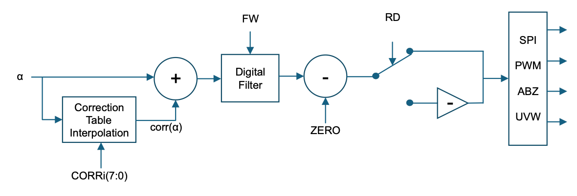
Figure 2: Block Diagram of the Digital Signal Treatment

HOW TO GENERATE THE CALIBRATION TABLE

Summary

Creating the calibration table involves measuring the full-turn error curve as a function of the raw angle (α) and selecting the negative value of the error at each lookup angle (a_i, where i ranges from 0 to 31).

Side-Shaft Considerations

In a side-shaft configuration, the error tends to be larger than in end-of-shaft configurations. Therefore, the BCT parameter must be adjusted first to ensure that the error curve remains within the valid CORRᵢ range — specifically, within ±11.25°.

To estimate a suitable BCT value, it is convenient to begin with MPS’s online magnetic field simulation tool. However, this initial estimate should be validated experimentally by fine-tuning the BCT values to minimize the error curve.

If mechanical tolerances and system-to-system variations are minimal, the experimentally determined BCT value can be the same across all sensors sharing the same mechanical set-up. Use the simulation tool to verify whether mechanical tolerances introduce errors exceeding ±11.25°. If they do, a unique BCT must be configured for each individual system.

Methods to Measure the Error Curve

There are two primary approaches to obtain the error curve:

• Method A: Using a high-precision reference encoder
• Method B: Rotating the magnet at a constant speed when there is no reference encoder.

Method A is straightforward, as the true angle is given by the encoder. In method B, the sensor’s output is acquired as a function of time. It is based on the assumption that the true angle is proportional to the time. To accurately determine the speed, use the time needed for multiple rotations.

Set-Up Accuracy Requirements

For both methods, the magnet’s positioning accuracy must significantly exceed the target calibration accuracy (typically, by a factor of 5 to 10).

In Method A, accuracy depends on the reference encoder’s precision.

In Method B, accuracy is influenced by the speed ripple, which is the variation in rotational speed.

In general, the speed ripple ratio (the ripple divided by the nominal speed) must be much smaller than the target angular accuracy, which is expressed in radians.

If the speed ripple is cause by motor cogging, then the error can be increased or decreased by changing the rotating shaft’s inertia. The resulting error (err_SR) can be calculated with Equation (5):

Where f_ROT is the magnet rotation frequency, τ_RIP is the motor’s torque ripple, and I is the shaft’s total moment of inertia.

Measurement of the Error Curve and Conditioning

The error curve (err) represents the deviation between the sensor’s output and the true angular position, as estimated with Equation (6):

If the calibration table is empty (corr_i = 0 for all i) then the sensor’s output is equal to the raw angle, and err can be calculated with Equation (7):

Therefore, measuring the error curve involves measuring the sensor’s output across a complete revolution with the maximum possible accuracy.

Setting the Reference Zero

The primary objective for calibration is to correct the linearity, not to define an absolute zero angle. Shifting the zero point merely offsets the sensor’s response curve by a constant and does not affect linearity. The application-specific zero angle should be configured after calibration.

As a result, the zero position of the reference angle (α_REF) is arbitrary and does not influence the correction. What matters is that no individual error value (err) exceeds the correction range of ±11.25°.

To ensure this, it is good practice to center the error curve around zero by subtracting its common-mode component. err_CENTERED can be estimated with Equation (8):

For N discrete error samples (err_j) that are approximatively evenly spaced across one full revolution, the centered error can be calculated with Equation (9):

If the dataset does not span a complete turn, a practical alternative is to subtract the median value of the error range. In this scenario, err_CENTERED,j can be estimated with Equation (10):

How to Minimize the Noise

To generate the optimal correction table, it is essential to isolate systematic errors — those that calibration can compensate — from the random noise. The less noisy the error curve, the more precise the correction values. Two calibration approaches, each with specific strategies for noise suppression, are described below.

1. Calibration using a Reference Encoder (Method A): This method typically involves slow, step-wise measurements (“stop-and-go”), allowing for effective noise filtering.

Noise can be minimized by selecting a large filter window, but one should ensure that the filter time constant (τ) is significantly shorter than the stationary time at each measurement point. This allows the sensor’s output to stabilize before recording.

One way to determine whether the stationary time is sufficient is to ensure that the following condition is fulfilled. After moving by a step (α_STEP), one must wait for the sensor’s output change (Δα_OUT(t)) to equal the step size plus or minus a tolerance much smaller than the target accuracy. The output must satisfy the condition calculated with Equation (11):

For instance, if the measurement step (α_STEP) is 10°, a calibration with an accuracy of 0.1° must fulfill the relationship estimated with Equation (12):

According to Figure 3 on page 9, this condition is met when the waiting time is longer than 9 times the filter time constant. The datasheet provides the time constants (τ) for every filter window and the resulting noise level expressed in noise-free resolution. The step response (as a function of time after the step) is expressed in integers of the filter constant to show the convergence of the sensor output to its final value.

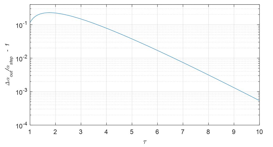
Figure 3: Step Response ^{(1) (2)}

Notes:

1. Since the filter window does not affect the systematic error, calibration can be accomplished with a large window, even if normal operation uses a smaller window.
2. A long filter time and single sample is equivalent to a short filter time and multiple samples, provided that the sampling interval exceeds the filter time constant.

2. Calibration during Constant-Speed Rotation (Method B): When calibrating with constant-speed rotation, measurements are taken on the fly.

As with the previous case (referring to calibration with a reference encoder), the filter time constant should be adjusted to be as large as possible to suppress noise without distorting the error curve. A large filter window can attenuate the error curve features that the measurement is supposed to capture. This means that filter time constant (τ) must be much smaller than half the period of the highest harmonic component, as calculated with Equation (13):

Where T is magnet’s rotation period, f_ROT is magnet’s rotation frequency, and D is the highest harmonic degree of the error curve features.

If a large filter window cannot be used, averaging should be executed by recording the error across multiple rotations. Since raw angles are modulo one revolution, measurements naturally fold into a single cycle.

Precise calibration requires precise knowledge of the magnet’s position. In Method B, the acquisition time and rotation speed are used to infer the magnet position. This approach is valid when the rotation speed remains constant, which is a reasonable assumption if the shaft moment of inertia is such that the speed ripple error (err_SR) in Equation (5) on page 7 is small.

Estimating Rotation Speed via Zero Crossings

Motor control signals typically lack the precision needed to reliably determine rotation speed. Instead, it is recommended to estimate the average speed directly from the sensor data — for example, by detecting zero crossings in the signal. Expressing acquisition times in terms of rotation period ratios eliminates the need for precisely knowing the absolute frequency of the initiator’s device clock.

Improving Speed Estimation with Multiple Rotations

Measuring across several full rotations enhances speed estimate accuracy. The uncertainty in rotation speed becomes proportional to the ratio of the sampling interval to the total duration of the measured revolutions.

Regarding the noise spectrum, both Method A and Method B rely on filtering or averaging. Since the MA600A exhibits some 1/f noise in addition to white noise, filtering yields less noise reduction than predicted under the Gaussian assumption. Specifically, increasing the acquisition time by a factor of four does not guarantee a two-fold reduction in noise level.

Data Interpolation

On the chip, the input of the calibration block is the raw angle (α); therefore the function to interpolate is the err as a function of α, and not a function of the real angle (α_REF). This means that the error curve must be represented by the experimental dataset [α_j, err_j] (with j = 1…N). Figure 4 shows an example in which N = 100. Consequently, even if the mechanical angles (α_REF) are evenly spaced, the raw data points (α_j) shown on the x-axis in Figure 4 are not evenly spaced.

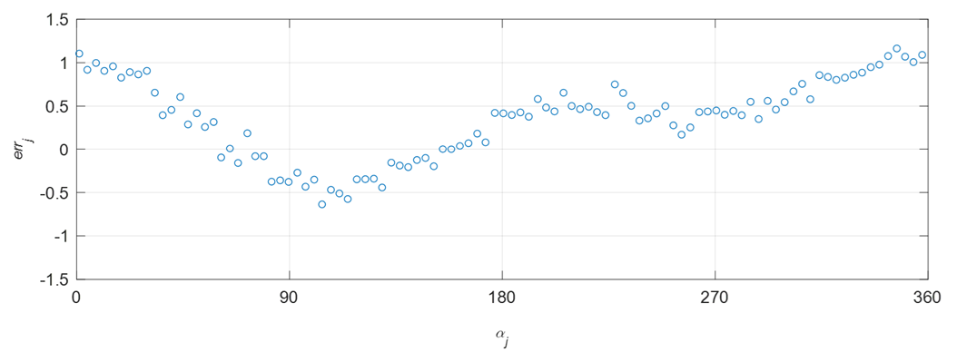
Figure 4: Example of Error Data

The goal of interpolation is to obtain the best estimate of the correction points (corr_i) out of the dataset for [α_j, err_j]. With methods A and B, we obtain an error curve where the raw output points are, in general, different from the lookup angles (a_i). Note that in principle, with method A, it is possible to search for the raw angle corresponding to a_i, but this is a tedious operation that does not provide the best estimate for correction because it does not suppress the residual noise. It is recommended to extract the lookup corrections (corr_i) from a fit of the complete error dataset.

Harmonic Fit

There are several ways to interpolate data while minimizing noise. One proposed way relies on the hypothesis that the error curve possesses some kind of regularity and uses a mathematical fit to calculate the correction at a_i points. The assumption, which is valid in most cases with a clean magnetic environment, is that the error curve as a function of the reference angle (α_REF) is a sum of a 1st, 2nd, and 4th harmonics.

Since the error curve is modified when expressed as a function of the raw angle (α_j), the harmonic content tends to increase when nonlinearity is large. The more we limit the harmonic content, the more we suppress noise. Typically, in end-of-shaft configurations, we can reasonably expect a harmonic content up to degree (D) of 4, and in side-shaft configurations up to a D of 8.

The harmonic fit of the error curve (f(α)) can be obtained simply by taking the first D terms of the Fourier series. It can be estimated with Equation (14):

Where H₀, H_x,k and H_y,k are the Fourier coefficients of the continuous error curve (err(α)) that can be calculated with Equation (15), Equation (16), and Equation (17), respectively:

For the discrete dataset, [α_j, err_j] is not evenly spaced. In this scenario, the Fourier coefficients can be approximated by the trapeze method, as estimated with Equation (18), Equation (19), and Equation (20):

Where α_FT is the full turn angle, which is 360° if α_j are expressed in degrees and 2π if α_j are expressed in radians. Figure 5 shows a fit example, where the blue circles are the error data for err_j from Figure 4, and the solid red line is a fitting function (f) with a constant term of H₀; the 1st and 2nd harmonic terms are H_x,1, H_y,1, H_x,2, and H_y,2.

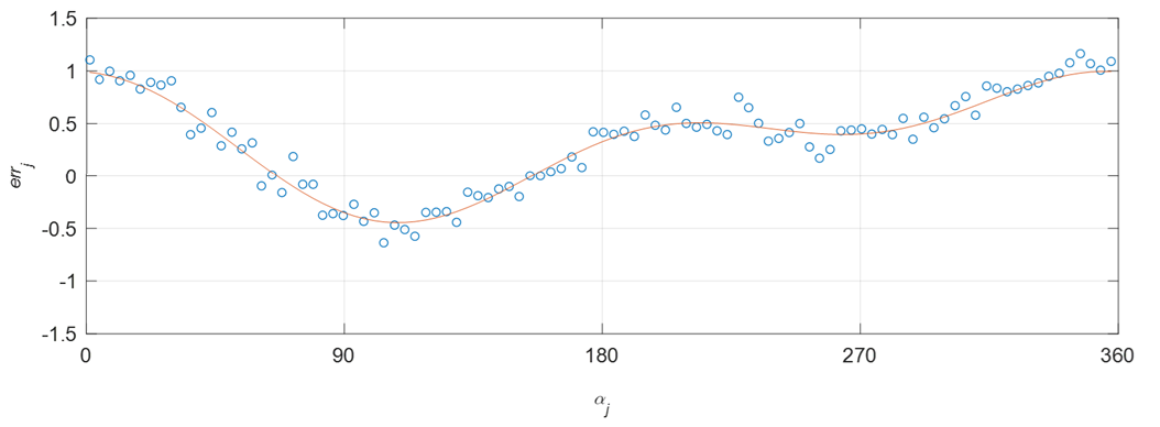
Figure 5: Fit Example

To verify the fit quality in an automated calibration procedure, it is useful to have a criterion to verify that data are fitted correctly. Various criteria can be applied to determine the quality of the fit, such as the coefficient of determination, which is denoted as R². A common feature among most of these criteria is the evaluation of the sum of squared residuals (SSR), which can be calculated with Equation (21):

Residual noise affects the SSR. Thus, setting the pass/fail criterion requires knowledge of the SSR under normal noise conditions. One approach to defining the criterion is to measure the SSR using a test case where the residual noise matches expectations and the fitting curve captures the features of the error curve that one would like to suppress.

Once the fitting function (f(α)) is determined, the 32 correction values are calculated by evaluating the inverse of the error at the lookup angles (a_i). In this scenario, corr_i can be estimated with Equation (22):

Table Construction

Once the 32 corr_i have been determined, the conversion into the lookup table format can be accomplished through the following relationships.

If corr_i ≥ 0 then, CORRi(7:0) can be calculated with Equation (23):

If corr_i < 0, then CORRi(7:0) can be estimated with Equation (24):

Where α_FT is the full turn angle, which is 360° if corr_i are expressed in degrees and 2π if corr_i are expressed in radians.

Table 3 shows an example of lookup corrections and the conversion to the integer format ready to be stored in the memory.

Table 3: Example of Lookup Table Construction

i	ai	corri	CORRi (7:0)
	Degrees	Degrees	Dec
0	0	0.11	1
1	11.250	-0.34	252
2	22.5	-1.29	243
…	…	…	…
30	337.5	0.64	7
31	348.75	0.33	4

Lookup Table Loading

The table is loaded to the MA600A memory in two steps: first, by writing the CORRi values into the volatile registers; second, by transferring the registers content to the NVM. A serial peripheral interface (SPI) is used to communicate with the sensor.

Write CORRi Values in the Volatile Registers

To store the CORRi values in the registers, use the Write Register command composed of three 16-bit words 32 times (see Table 4).

Table 4: Command to Write One 8-Bit Value CORRi into the Corresponding Register

	1st 16-Bit Word	2nd 16-Bit Word		3rd 16-Bit Word
COPI	0xEA54	8-bit address (0x20 to 0x3F)	8-bit CORRi	0x0000
CIPO	Angle out	Undefined data		Angle out	8-bit CORRi

During the second half of the third 16-bit word, the MA600A responds by reading back the transmitted 8-bit CORRi value. As explained in the datasheet, registers are grouped in sets called “blocks”. The 32 registers (0x20~0x3F) containing the lookup table form “Block 1”.

At this stage, once the lookup registers are filled, the sensor automatically corrects the output, but the lookup table would be erased if the sensor turns off. To keep the lookup values after a shutdown, proceed with the next step.

Store to the NVM

The full content of Block 1, with the 32 correction values, can be transferred to the NVM by a single command consisting of two 16-bit words (see Table 5).

Table 5: Command to Store the 32 Registers of Block 1 to the NVM

	1st 16-Bit Word	2nd 16-Bit Word
COPI	0xEA55	0xEA01
CIPO	Angle out	Angle out

TYPICAL SEQUENCE OF OPERATIONS

1. Clear the ZERO register.
2. Set RD to zero.
3. For end-of-shaft configurations, set the BCT value to zero. For side-shaft configurations, set the final BCT value.
4. Rotate the magnet and acquire error data.
5. Calculate the correction values (CORRi).
6. Write the calibration register.
7. Check that calibration works and the error is suppressed.
8. Load the table to the NVM.
9. Adjust RD.
10. Adjust ZERO.
11. Store ZERO, RD, and BCT to the NVM.