Understanding Frequency Spread Spectrum: The Benefits and Limitations of Using FSS in Modern SMPS Designs

Florian Seliger

Get valuable resources straight to your inbox - sent out once per month

We value your privacy

Abstract

Modern passenger vehicles are not only made to carry passengers from one destination to the next — they must also function as communication tools, TVs, home cinema sets, LED illumination centers, and even massage parlors. The customer’s focus is changing from purely driving characteristics (e.g. horsepower and acceleration) to include entertainment systems, such as the size of the multimedia touchscreens and the ability to access mobile networks.

The vehicle of tomorrow must be able to connect to social media, stream UHD videos, and keep passengers online, as well as communicate with other vehicles, infrastructure, and pedestrians to enable autonomous driving. On top of that, these cars must maintain older features such as classic electrical control units (ECUs) for features like radio tuners and GPS navigation. This leads to a rising number of ECUs.

The rise of vehicle electrification requires solutions with efficient and powerful power conversion. These solutions are expected to have small form factors for power supplies. Having excellent efficiency and a small form factor requires high switching frequencies as well as very fast switching flanks on the switching point of the switch-mode power supply (SMPS), which poses challenges for EMC engineers.

This article will explore how frequency spread spectrum (FSS) can be used to effectively reduce the EMI spectrum of a power supply in specific frequency bands, as well as related physical limitations.

Understanding Frequency Spread Spectrum (FSS)

To understand how FSS works, let’s look at the spectrum of a traditional SMPS such as the MPQ4371-AEC1. The MPQ4371-AEC1 is an automotive buck regulator that can achieve up to 11A of continuous output current (I_OUT) with zero-delay PWM (ZDP^TM) control and a switching frequency (f_SW) up to 2.5MHz.

Figure 1 shows the spectrum of this SMPS when the main f_SW is set to 2.2MHz. The corresponding harmonics can be calculated as (n x f_SW), where n is the corresponding harmonic.

Figure 1: Spectrum of a Traditional SMPS

The power of the harmonics decreases with higher measurement frequencies, and it disappears in the noise floor at about 400MHz. Each peak in the spectrum (calculated with n x f_SW) is shown with the resolution bandwidth (RBW) and the filter type used by the spectrum analyzer.

The RBW filter is defined by the minimum and maximum frequency, as well as the filter order. RBW determines the settling time (t_S) for the RBW filter, calculated with Equation (1):

$$t_s=\frac{1}{RBW}$$

Figure 2 shows a traditional RBW filter of a spectrum or signal analyzer.

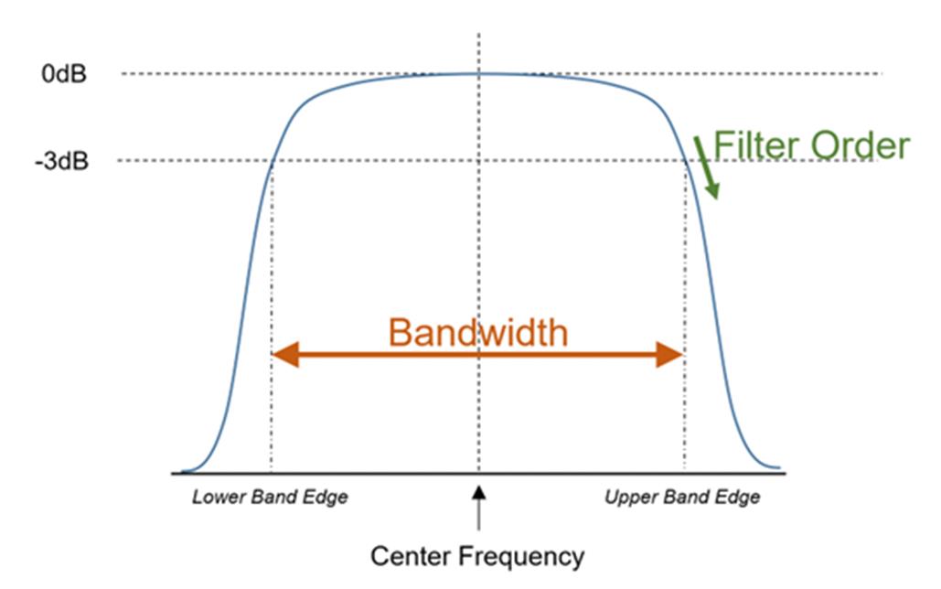
Figure 2: RBW Filter Characteristics

By measuring a spectrum, the spectrum analyzer sweeps through the defined frequency area. Whenever there is a peak inside the RBW filter, this specific frequency is shown in the scope (see Figure 3). This provides the possibility to move power from each specific harmonic inside the area between the peaks.

Figure 3: Resolution Bandwidth Filter and Switching Frequency in the Spectral Area

Figure 3 shows that a higher RBW combined with a smaller f_SW will move the spectrum closer together. This means the energy of the harmonics can only be transferred to a smaller area. Theoretically, if all the energy of the peaks is transferred into white noise, the attenuation (α) of each specific peak is linked to f_SW and RBW, estimated with Equation (2):

$$α=10 x log (\frac{RBW}{f_{SW}})$$

Figure 4 shows the relationship between the maximum theoretical attenuation, which can be achieved via FSS, alongside the corresponding RBW and f_SW. As an example, assume that the SMPS’s f_SW is 0.5MHz, and the RBW is 120kHz; the maximum attenuation that can be achieved with FSS is 6.2dB.

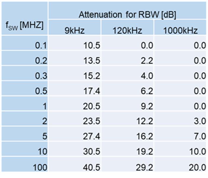
Figure 4: Maximum Possible Theoretical Attenuation for FSS

Transforming a Specific Spectrum to Frequency Spread Spectrum (FSS)

To transform the SMPS’s original spectrum to FSS, we must dither around the original switching frequency.

Figure 5: Modulation Signal for FSS Showing the Context of f_SPAN and f_MOD

To dither around the original switching frequency, consider the following:

t_S: The RBW’s settling time must be considered. If the time for the frequency to change (the modulation frequency, or f_MOD) is longer than t_S, there is no achievable attenuation with FSS.
RBW: Because if the dither frequency (f_SPAN) is smaller than the RBW, the frequency dithers within the filter’s bandwidth, and the attenuation with FSS is zero.

When considering the two rules above, it can be concluded that f_SPAN must exceed the RBW, calculated with Equation (3):

$$f_{SPAN}>RBW$$

Meanwhile, f_MOD must exceed the inverse of t_S, estimated with Equation (4):

$$f_{MOD}>\frac {1}{t_s}, \text{with} t_s=\frac{1}{RBW}$$

The frequency change (f_SPAN x f_MOD) can be calculated with Equation (5):

$$\text{Frequency Change}=f_{SPAN} \times f_{MOD} > RBW^2 [\frac{Hz}{s}]$$

Table 1 shows the frequency change values to achieve FSS within specific RBWs.

Table 1: Frequency Changes to Achieve Attenuation

RBW	Settling Time	Minimum Frequency Change
9kHz	111µs	81MHz/s
120kHz	8.33µs	14.4GHz/s
1000kHz	1µs	1THz/s

To generate a white noise signal and be compliant with the two rules above, we need to dither from zero to infinity within a period very close to zero. As this is technically impossible, the dither frequency (f_SPAN) should be between 10% and 20% of the original f_SW. This will provide enough f_SPAN to ensure a good attenuation, and it will keep the SMPS at a stable operating point.

Real measurements show that the attenuation with FSS is most effective when the modulation frequency (f_MOD) is almost equal to the spectrum analyzer’s RBW.

For example, consider a scenario where f_SW is 2MHz and f_SPAN is 20%. Table 2 shows f_MOD and the frequency change for this scenario.

Table 2: Frequency Change for Given Working Areas

Modulation Frequency (f_MOD)	Header
9kHz	3.6GHz/s
120kHz	48GHz/s

By comparing Table 1 and 2, it can be observed that it is possible to achieve great attenuation for an RWB of 9kHz with an f_MOD of 9kHz. However, the attenuation with an RBW of 120kHz is 0 since the frequency change is too slow. To achieve reasonable attenuation for a 120kHz RBW, we must increase the FSS frequency.

Because FSS is always modulated to the SMPS’s switching frequency, high harmonics will automatically reach a high frequency change at their dedicated frequency (see Table 3).

Table 3: Corresponding Frequency Change for the SMPS’s Harmonics

Harmonic	Spectral Frequency	f_MOD	f_SPAN (20%)	Frequency Change
f_SW	2MHz	9KHz	400kHz	3.6GHz/s
Second harmonic	4MHz	9KHz	800kHz	7.2GHz/s
Third harmonic	6MHz	9KHz	1200kHz	10.8GHz/s
Fourth harmonic	8MHz	9KHz	1600kHz	14.4GHz/s

Modulation Waveforms

After establishing the correlation between f_MOD and f_SPAN, we can consider the modulation waveform. Because the frequency change during normal operation should be linear, the easiest way to modulate FSS is by using a triangular modulation signal (see Figure 5). This is simple to implement, but at the signal’s edges, the frequency change within a specific timeframe is half of the frequency change during the rising or falling flank (f / 2).

To prevent this, it is possible to use a sawtooth waveform, where the frequency change is linear while ramping. After receiving the maximum f_SW, the SMPS changes from the maximum to minimum f_SW within one switching cycle. However, this can cause control loop instability and output voltage (V_OUT) undershoot or overshoot.

Therefore, mixing different waveforms (e.g. the “Hershey’s Kiss” waveform or a stepped triangular waveform) are ways to optimize attenuation while maintaining SMPS stability.

Figure 5 shows the different FSS modulation waveforms.

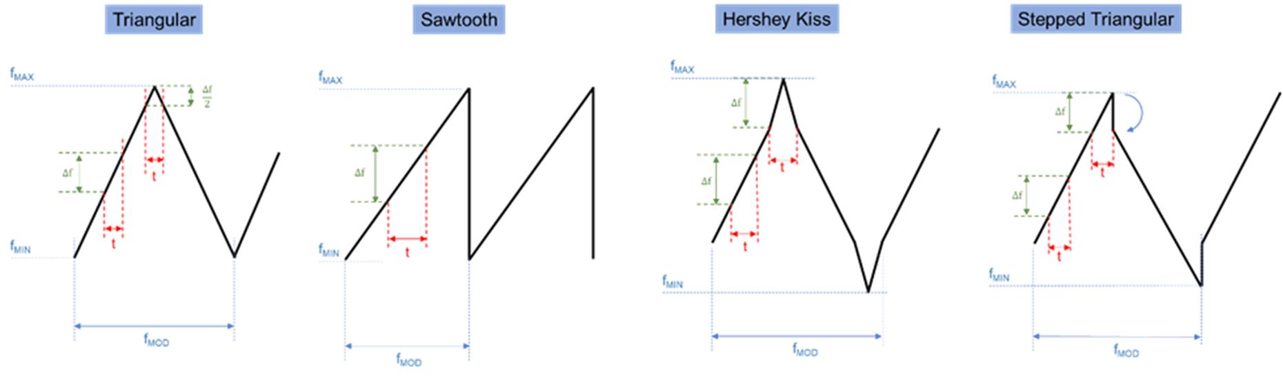
Figure 6: Different FSS Modulation Waveforms

All of these waveforms have one thing in common: They can only be used with one specific modulation frequency (f_MOD).

From the rules in the paragraph above, f_MOD should be within the frequency area of the RBW to achieve the best possible attenuation. When checking the CISPR 25 norm, there are two very critical frequency areas for SMPS developers:

The rod-antenna measurement, which goes from 150kHz to 30MHz with an RBW of 9kHz.
The biconical-antenna measurement, which goes from 30MHz to 300MHz and has its toughest limits with an RBW of 120kHz.

As these two measurements use two different RBWs, the FSS f_MOD can only be optimized for one specific frequency area.

To optimize FSS for the full spectrum, the MPQ4371-AEC1 offers dual-FSS modulation (see Figure 7).

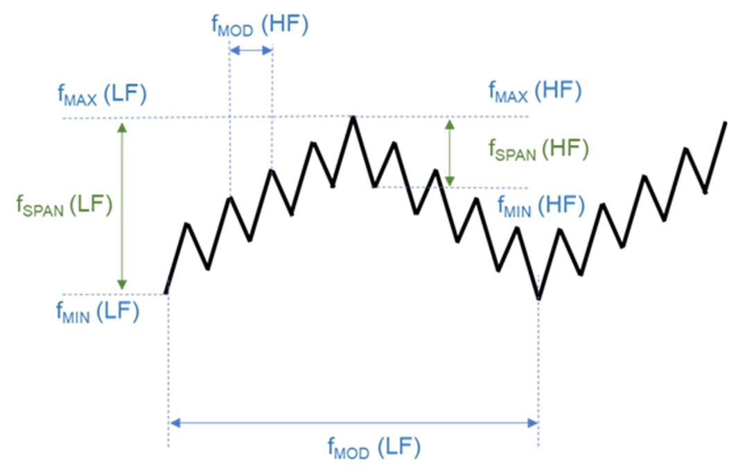
Figure 7: MPQ4371-AEC1 Dual-FSS Modulation Waveform

Using this modulation waveform provides the benefits of FSS within the low-frequency (LF) and high-frequency (HF) spectrum. The main carrier (f_MOD(LF)) has a frequency of 15kHz, which is optimized to achieve an attenuation on the SMPS spectrum with the rod-antenna measurement. Ideally, f_MOD(LF) should have a frequency of 9kHz, but this frequency can cause audible noise from the SMPS. To avoid this, f_MOD(LF) can be increased to 15kHz. This gives nearly the same attenuation as the 9kHz modulation frequency and avoids audible noise. The second frequency is modulated on the carrier frequency with 120kHz, which provides an additional attenuation for the biconical antenna measurement. Using dual-FSS modulation provides the possibility to tune the specific modulation frequency’s f_SPAN for each given use case. The MPQ4371-AEC1 provides eight different FSS options to allow for further fine-tuning (see Table 4).

Table 4: FSS Options for the MPQ4371-AEC1

f_SPAN Options	f_MOD(LF) (15kHz)	f_MOD(HF) (120kHz)
f_SPAN 1	-	-
f_SPAN 2	10%	-
f_SPAN 3	6.2%	-
f_SPAN 4	8.6%	2.5%
f_SPAN 5	6.2%	2.5%
f_SPAN 6	6.2%	4.3%
f_SPAN 7	4.8%	2.5%
f_SPAN 8	4.8%	4.3%

Practical Measurements

To show the effects of the different types of FSS, we can compare different versions of the MPQ4371-AEC1 on a real evaluation board with identical settings. The standard evaluation board for the MPQ4371-AEC1 ⁽¹⁾ was used in a CISPR 25 EMC chamber, and the measured frequency range was between 150kHz and 1GHz. To compare the effects of FSS, three modes were tested:

The MPQ4371-AEC1 without FSS (green trace)
The MPQ4371-AEC1 with 15kHz FSS and a ±10% span (blue trace)
The MPQ4371-AEC1 with dual-FSS: 15kHz FSS and a ±6.2% span, and 120kHz FSS with a ±2.5% span (yellow trace)

Note:
1) Contact an MPS FAE for details on this evaluation board.

In all three scenarios, the MPQ4371 ran with a 2.2MHz f_SW and a 3A load. Figure 8 shows the measurements captured via the rod-antenna method with an RBW of 9kHz.

Figure 8: EMC Measurements for Three Different Types of FSS (Rod-Antenna)

Figure 9 shows the EMC spectrum in the frequency area between 30MHz and 1GHz with a RBW of 120kHz.

Figure 9: EMC Measurements for Three Different Types of FSS (Biconical and Log-Periodic Antenna)

Figure 8 and Figure 9 show that FSS can make a huge difference on the SMPS’s frequency spectrum. Especially for the rod-antenna measurement, FSS can effectively reduce the peaks at the fundamental switching frequency and the first harmonics. In this scenario, a maximum attenuation of 14dB is achieved.

For the rod-antenna measurement, the single 15kHz FSS is more effective than the dual-FSS method, since the frequency span is bigger for that modulation (10% with single-FSS vs. 6.2% with dual-FSS).

However, higher frequencies benefit from the dual-FSS method, especially in the 40MHz to 140MHz range. Dual-FSS provides an additional benefit of up to 3dB since f_MOD stays within the RBW.

Conclusion

Frequency spread spectrum is an effective method to provide attenuation to the spectrum of an SMPS. Care must be taken regarding the modulation frequency and the frequency span, as these are two critical limitations that can result in no attenuation at all. In addition, the modulation waveform plays a role, since using single-FSS or dual-FSS influences different frequency areas, whereas each specific waveform (e.g. triangular or sawtooth) also influences the stability of the SMPS.

Ultimately, using FSS should be a case-by-case decision. FSS should be tuned such that the most sensitive frequency areas provide the most attenuation within the SMPS spectrum, which makes devices such as the MPQ4371-AEC1 ideal, as it provides up to 8 different FSS options. Visit the MPS website to find an automotive-grade step-down converter that can meet you design needs.