Magnetic Angle Sensors: Resolution Explained

Carmine Fiore

Serge Reymond

Get valuable resources straight to your inbox - sent out once per month

We value your privacy

Introduction

Because optical encoders are functionally similar, “resolution” is often used as a main characteristic for magnetic encoders (a device providing the angle of a magnet attached to a mechanical shaft, under a digital form). Resolution is a key parameter since it indicates the smallest angle that the sensor is capable of resolving. Unfortunately, when comparing products, users may often be misled, as resolution is defined in different ways in both commercial and technical documents.

This article proposes the most meaningful way to define resolution, such that it can be consistently determined across different products’ datasheets. We will also show that for magnetic encoders, resolution alone is not sufficient to adequately compare products. Sensor bandwidth, which is often absent in many magnetic position sensor datasheets, is also required to compare magnetic angle sensors.

Measurement Error

Before defining resolution, it is important to clarify some points related to measurement error. A measurement error is defined as the difference between the measured value of a quantity and its true value. This error can be divided in two components, described below:

Systematic (or bias) error: Systematic error is the component that stays constant across multiple measurements performed under the same conditions. This error can be estimated as the difference between the average of a large number of measurements, and the true value of the measurand.
Random error: Random error is the total error minus the systematic error. It accounts for the unpredictable variations in a group of measurements performed under the same conditions.

Figure 1 shows the different combinations of random and systematic error. There are three groups of measurements, with different amounts of random and systematic error. Group A has a larger random error, group B has a larger systematic error, and group C has similar random and systematic errors.

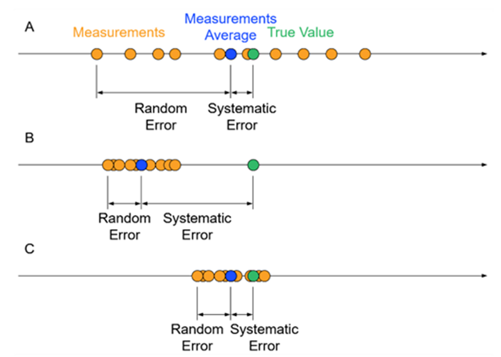
Figure 1: Combinations of Random and Systematic Error

In magnetic angle sensor datasheets, the systematic and random errors are expressed as INL and resolution, respectively. For simplicity, this article will assume that the sensor has no systematic error, which means that the average value is the true value.

Standard Deviation and Confidence

A metric that can be used to quantify the amount of random error in a measurement is standard deviation (σ). In statistics, σ measures the dispersion of a set of samples around their average. The higher the dispersion, the higher the σ. This parameter is also referred to as the root-mean-square (RMS) noise.

Sets of measurements often follow a bell-shaped curve distribution, also referred to as a Gaussian or normal curve (see Figure 2). This is the case when the random variation does not depend on the past error. The Gaussian curve peaks at the measurements’ average (µ), and σ characterizes its width. If the total area under the Gaussian curve is normalized to 1, then the area delimited by a range of values [a1, a2] is the probability that the result of a measurement falls somewhere between a1 and a2. The larger the range, the greater the confidence that a single measurement falls into that range.

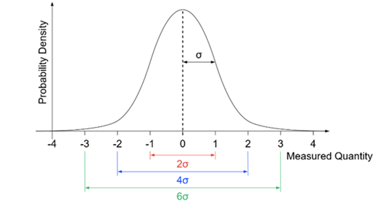
Figure 2: Gaussian Distribution with µ = 0 and σ = 1

Table 1 lists the probability or confidence that the measurement is included into the range [µ - nσ, µ + nσ].

Table 1: Confidence Factor for Several Values of n

n	Confidence (%)
1	68.269
2	95.450
3	99.730
4	99.993

Defining Resolution

The US National Institute of Standards and Technology (NIST) defines resolution as “the ability of the measurement system to detect and faithfully indicate small changes in the characteristic of the measurement result”.

Resolution is then the smallest interval that an instrument can detect. To determine this interval, this article will assume that the distribution of random errors follows the Gaussian distribution. This leads to a question: how far apart should two angles be, to be able to distinguish both angles with a reasonably high probability?

When the distance between the two angles is smaller than 6σ, the two noise distributions centered on the angles significantly overlap (denoted as “A” in Figure 3). If the result of the measurement falls in the overlap region, it is impossible to know if the true angle is angle a1 or a2. It is only when the distance between the two angles is equal to or larger than 6σ that a single measurement can distinguish between these two points with a confidence equal to or higher than 99.73% (denoted as “B” in Figure 3). Therefore, the sensor’s resolution is an interval of 6σ.

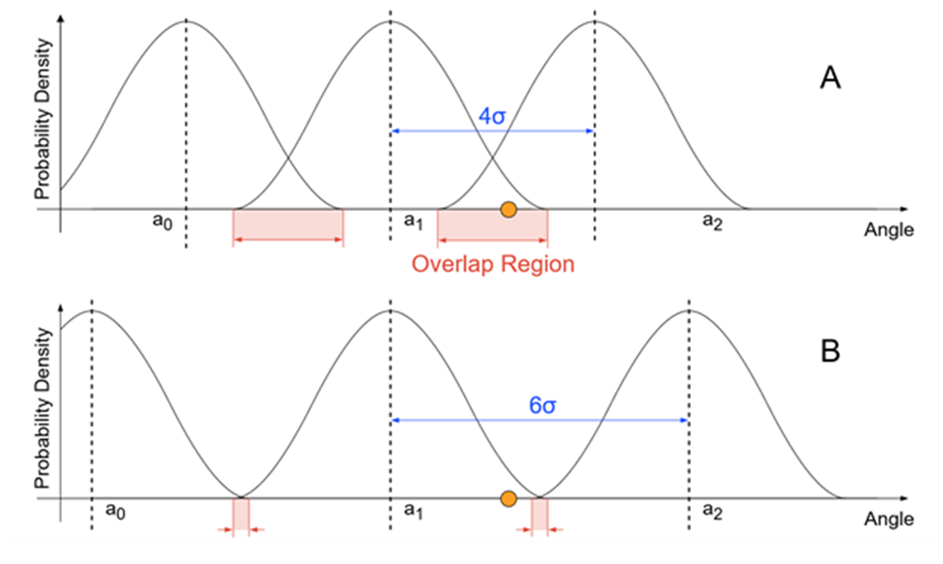
Figure 3: Sample Contained in the 6σ Intervals Centered on µ1

Analog-to-Digital (AD) Conversion

Generally, the output of position sensors is given in a digital format — for example, it may be provided through an ABZ or SPI interface. In this scenario, the analog signal from the magnetic sensor must be digitized. Figure 4 shows a simplified block diagram of a digital magnetic angle sensor. Note that the diagram includes a filter block, which will be further discussed in the next section.

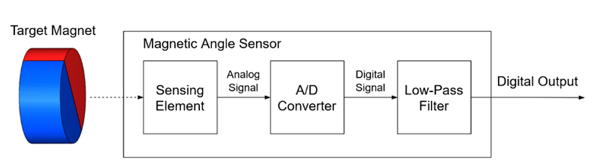
Figure 4: Digital Magnetic Angle Sensor

The step size for AD conversion — namely the range of values in the analog domain divided by the number of steps in the digital domain — is often wrongly interpreted as the sensor’s resolution. This interpretation is only correct when the peak-to-peak noise of the analog signal is smaller than the step size of the AD conversion.

However, this is not true in most scenarios. The peak-to-peak noise of the analog signal often exceeds the AD step, so it appears at the sensor’s digital output as random flicker of the output’s least significant bits (LSBs). This is why analog-to-digital converter (ADC) manufacturers defined indicators such as “noise-free resolution” or “peak-to-peak resolution.”

Figure 5 shows how noise is carried from the analog domain to the digital domain. In this example, the step size is 1, while the peak-to-peak noise is 6. In addition, the continuous and discrete distributions are shown on the X-axis and Y-axis, respectively. Since the noise exceeds the digital step, decreasing the step size does not improve the resolution.

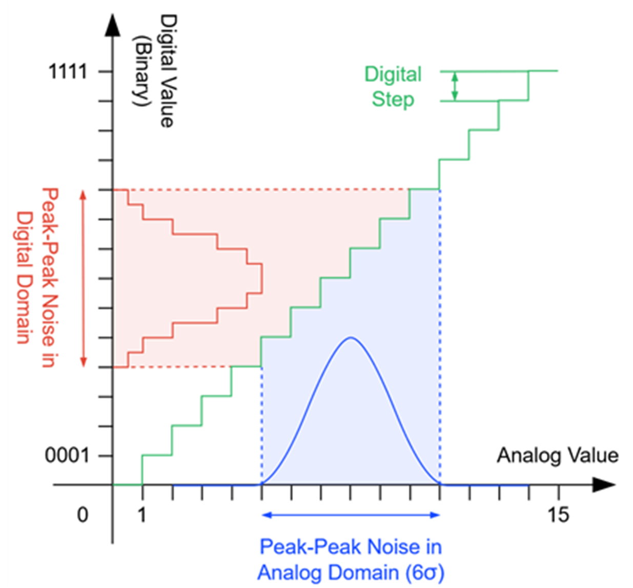
Figure 5: Noise in AD Conversion

When providing a measurement in a digital format, the resolution can be also expressed in bits, calculated with Equation (1):

$$resolution_{bit} = log_2 \frac {FS}{6 \sigma}$$

Where FS is the full scale of the quantity to be measured.

In the case of angle measurements, FS = 360°, which means the resolution can be estimated with Equation (2):

$$resolution_{bit} = log_2 \frac {360}{6 \sigma}$$

Bandwidth

When discussing sensor performance, a key parameter that is often overlooked is the bandwidth, also known as the cutoff frequency. Sensor bandwidth corresponds to a signal’s frequency range, which can be measured by the sensor. Signals with a frequency larger than the sensor bandwidth are attenuated. A detailed characterization of the sensor would require its transfer function under an analytical or graphical form. At the bare minimum, the cutoff frequency should be provided.

Figure 4 shows that a low-pass filter stage can be implemented in the sensor. This reduces the noise on the sensor output. In this case, the sensor bandwidth is the same as the filter’s bandwidth. If the noise distribution is Gaussian, decreasing the filter bandwidth by a factor of 4 decreases the noise by a factor 2, which increases the resolution by 1 bit. This means that information regarding the noise or resolution should correspond with information regarding the bandwidth.

A bandwidth that is too low for an application can have dramatic effects. If the sensor is used inside a control loop, the system may be unstable, and the motor may exhibit oscillations, noise, and/or loss of efficiency (see Figure 6). In this figure, R is the position reference, AM is the motor shaft angle, and AS is the sensor output. A common design rule is to have the filter bandwidth be at least ten times larger than the bandwidth of the control system or control loop.

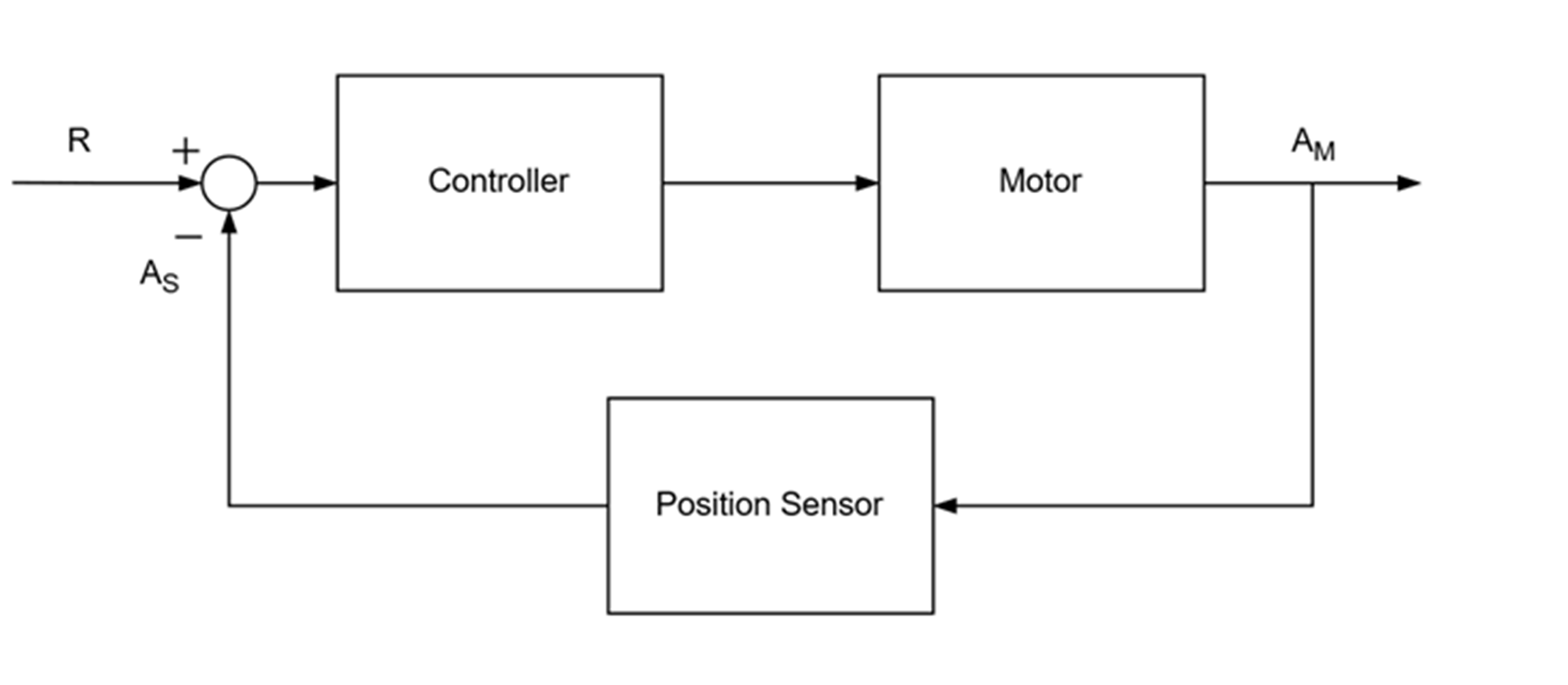
Figure 6: Motor Control Loop

Figure 7, Figure 8, and Figure 9 show the effects of a low-pass filter bandwidth (BW) on the angle measurement, the noise, and the control loop performance, respectively.

Figure 7 shows that the motor shaft angle and sensor output under a high BW filter almost overlap (denoted with the blue and green lines, respectively). Meanwhile, the sensor output with a lower BW filter is not able to follow the motor shaft position as accurately (denoted with the red line).

Figure 7: Effect of Different Filter Bandwidths on Sensor Output

Using a BW filter for the angle significantly reduces the noise (see Figure 8). As the bandwidth gets lower, the noise is more attenuated.

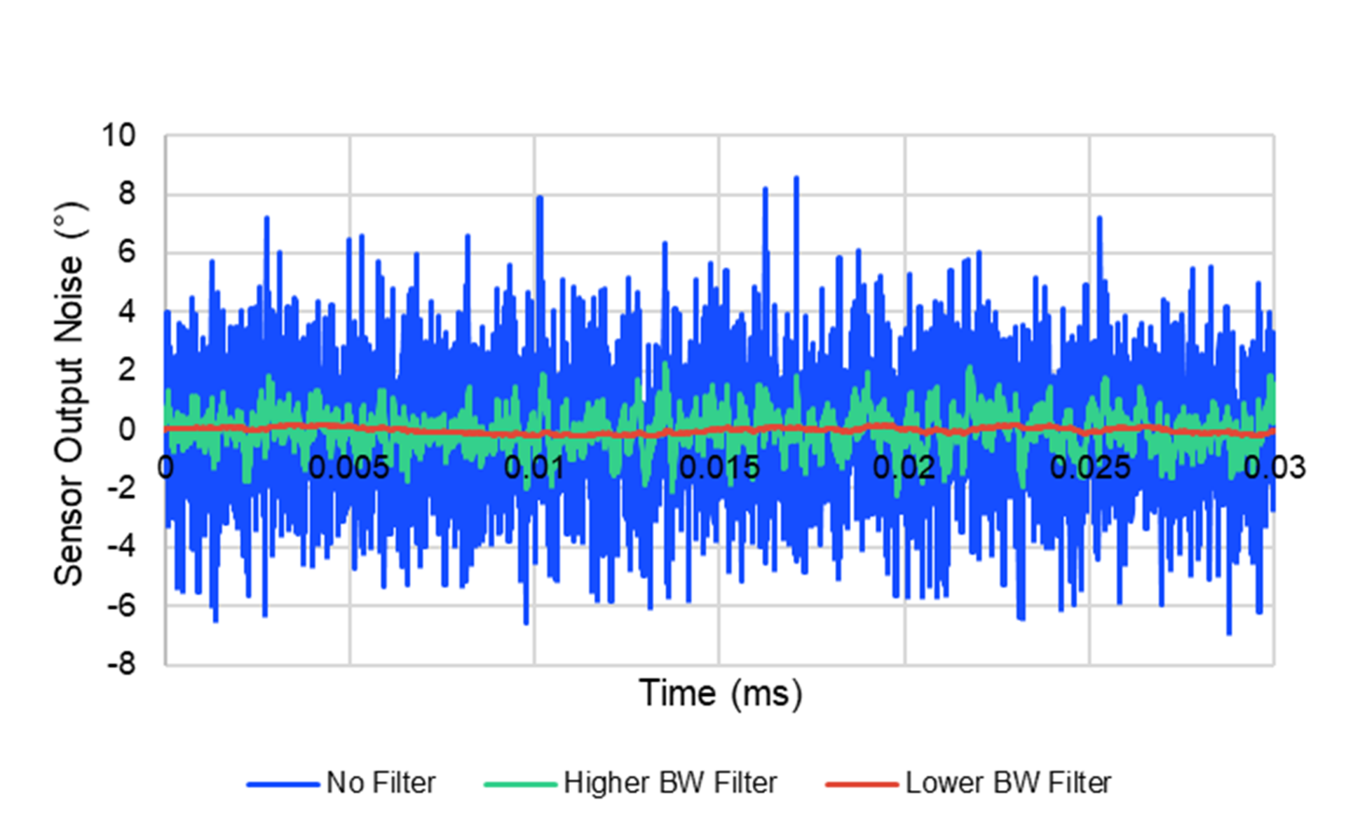
Figure 8: Effect of Different Filter Bandwidths on Sensor Output Noise

Figure 9 shows how different filter bandwidths affect motor control loop performance. If a filter has a lower bandwidth (denoted with the red line), then there is more overshoot and a longer settling time.

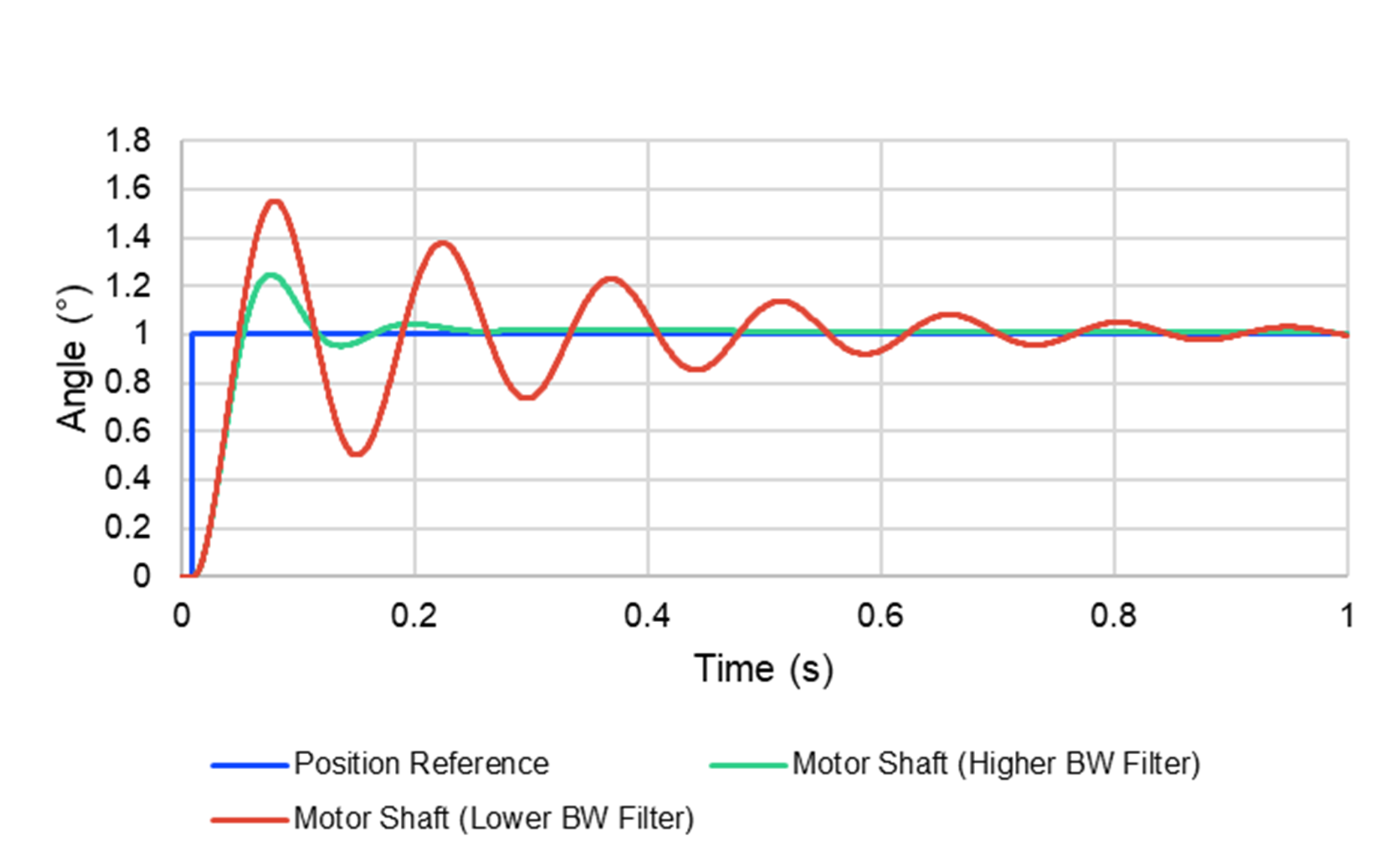
Figure 9: Motor Control Loop Performance

What to Look for in Datasheets

To ensure that a sensor is well-suited for your application, it is crucial to make a distinction between a digital step and the actual sensor resolution.

Often, when terms such as SPI resolution, AD resolution, and ABZ resolution are used, they specify how many bits are used for the digital representation of the measurement, but not the actual sensor resolution.

If specs such as RMS noise, peak-to-peak noise, angle noise, or noise density are included in the sensor datasheet, they are usually the most reliable source to obtain the sensor resolution. Then designers can use Equation (1) to calculate the resolution expressed in bits.

Table 2 shows an example from a datasheet. In this scenario, the resolution is misleading, since it is actually referring to the digital step. If the filter bandwidth is configurable, multiple noise values may be listed. Using the lowest noise value shown in the table, the resolution can be calculated with Equation (3):

$$resolution_{bit} = log_2 \frac {360}{6 \sigma} = log_2 \frac {360}{0.06} = 12.55$$

By comparing both resolution and the bandwidth, it is possible to determine the real performance differences between products. The filter bandwidth can be expressed through several parameters, such as the time constant, step response, or cutoff frequency. Table 2 shows an example using the filter time constant and filter cutoff frequency.

Table 2: Datasheet Example

Parameter	Symbol	Conditions	Min	Typ	Max	Unit
Resolution	RES		-	14	-	bits
RMS noise	σ	Filter setting = 0	0.004	0.08	0.14	deg
RMS noise	σ	Filter setting = 3	0.006	0.01	0.017	deg
Filter time constant	τ	Filter setting = 0	-	125	-	µs
Filter time constant	τ	Filter setting = 3	-	1000	-	µs
Filter cut-off frequency	f_CUTOFF	Filter setting = 0	-	3000	-	Hz
Filter cut-off frequency	f_CUTOFF	Filter setting = 3	-	350	-	Hz

MPS Sensors Performance

For many MPS angle sensors, the digital representation of the data is 16 bits; meanwhile, the resolution, sensing technique (Hall or TMR), and the filter bandwidth vary between parts.

Table 3 lists the resolution and bandwidth values for some sensors in the MagAlpha family. Note that some sensors have a configurable filter bandwidth, which allows them to be adapted to different application requirements.

Table 3: MagAlpha Family

Part Number	Resolution at 45m T (Bits)	Filter Bandwith (Hz)	Technology	Typical Application
MA600	14.5 to 12	150 to 13000	TMR	Closed loop position/speed control
MA732	14 to 9	23 to 6000	Hall	Closed loop position/speed control, general-purpose position sensors
MA330	14 to 9	23 to 6000	Hall	BLDC motor commutation
MAQ430	14 to 9	23 to 6000	Hall	Automotive
MA730	14	370	Hall	High-resolution encoders
MA704	10	3000	Hall	Closed loop position/speed control
MA780	12 to 8	39 to 160000	Hall	Low-power
MA800	8	90	Hall	HMI

The table also illustrates how the TMR sensing technique used inside the MA600 sensor helps achieve excellent resolution at higher bandwidths, when compared to Hall-based sensors.

Conclusion

The article explained the definition of resolution starting from the description of random error and the statistical concepts of standard deviation and confidence. It also clarified the difference between the digital representation (number of bits provided on the sensor output) and the resolution of the sensor measurement, in case this is provided in digital form.

By showing the effect of filtering, the article proved that both resolution and bandwidth must be considered to determine a product’s real performance. Finally, this article provided an example of a typical magnetic angle sensor datasheet to show how to correctly interpret the information contained in it.