Controlling Conducted EMI when Using Long Output Lines (Part II)

Get valuable resources straight to your inbox - sent out once per month

We value your privacy

Introduction

This article is part two in a three-part series exploring methods to analyze and improve excessive EMI under long-line loads. Part I reviewed the common-mode (CM) EMI model and considered the influence of electric field coupling and magnetic field coupling. Part II will discuss the transmission line effect on the output’s long-line impedance to ground, using a series of equations. Part III will review three EMI noise reduction methods to analyze and predict resonant peaks.

The Output’s Long-Line Impedance to Ground

Because the output line is long, consider the transmission line’s effect during high-frequency conduction. Note that this parameter is not typically relevant to power electronics engineers.

When the circuit’s wavelength corresponds to the frequency that will be investigated, note all relevant parameters. These parameters can include the voltage, current, and impedance, as well as any changes between the centralized parameters and the distributed parameters.

Figure 1 shows the system’s inductance, resistance, capacitance, and conductance, which can be examined for each transmission line segment.

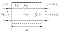
Figure 1: Transmission Line Model

The distribution of current and voltage on the transmission line can be calculated with Equation (1), respectively:.

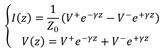
Where Z₀ is the transmission line’s characteristic impedance, and γ is the transmission constant. When the losses on the transmission line (R and G in Figure 1) are negligible, Z₀ can be estimated with Equation (2):

Then γ can be calculated with Equation (3):

Figure 2 shows that the output line has a geometric shape, which means that the parameters can be obtained using the electromagnetic field theory.

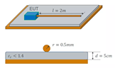
Figure 2: Geometric Model of an Output Line to Ground

If the loss is ignored, the capacitance can be estimated with Equation (4):

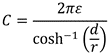
Where d is the distance between the line and the reference ground, r is the line’s radius, ε is the medium’s dielectric constant. The system’s inductance can be calculated with Equation (5):

Where µ is the medium’s magnetic permeability. For CM noise, the two output lines can be considered to be the same conductor.

Because there is no connection between the output line’s end and the reference ground, this system can be considered an approximate open circuit (where the end current is 0A). Thus, Equation (2) through Equation (5) can be substituted into Equation (1) to obtain the final output line’s current and voltage expressions. For output lines with a particular length (l), the final output line’s impedance (Z_OC) can be estimated using Equation (6):

Where ω is the angular frequency (2πf), and λ is the wavelength (1 / (f x (√LC)).

Depending on the nature of the trigonometric function for Equation (6), if l is an odd multiple of a quarter wavelength (e.g. 1/4λ or 3/4λ), the impedance undergoes series resonance, leading to a significant reduction in the EMI propagation path’s impedance. This reduces EMI peaks. If the length of the transmission line is 2m, then according to the actual situation, the frequencies corresponding to 1/4λ and 3/4λ are 31.6MHz and 95.1MHz, respectively. This calls back to the two EMI peaks in Figure 3 of Part I.

This theory is simple to verify with measurements. Figure 3 shows the ground impedance measurements of transmission lines with different lengths. For a 2m output line, the position of the impedance vibration peak is consistent with our previous calculation results, which also explains the resonant peak in the EMI measurement results. In addition, shorter output lines correspond with higher resonant frequencies.

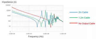
Figure 3: Ground Impedance Measurement Results for Different Lengths of Transmission Lines

Finally, the frequency corresponding to 1/4λ can be estimated using Equation (7):

Equation (7) confirms that the distance between the output line and the reference ground, as well as the line diameter, does not affect the resonance position. Resonance is only related to the output line’s length.

Conclusion

In this article, we completed our CM EMI model from Part I by calculating for the distribution of current and voltage, losses on the transmission line, inductance, capacitance, final output line impedance, and frequency. Part III will wrap up the series by analyzing the effect of noise reduction methods to successfully output long-line loads.