Basics of Modeling Control Systems in Simulation Environments

In power electronics engineering, modeling control systems in simulation environments is a fundamental practice. It allows engineers to design, analyze, and optimize control strategies before implementing them in physical systems. Analog and digital control systems can be modeled to better understand their behavior, predict performance, and detect possible issues early in the design process. The fundamental concepts and methodologies for modeling control systems are discussed in this section, with a focus on the value of simulation in the development of reliable and efficient power electronics systems.

The Importance of Control System Modeling

Control Systems in Power Electronics: Control systems are essential for controlling how power electronics devices operate and making sure they fulfill requirements including load management, voltage regulation, and current control. In power converters, motor drives, and other applications, control systems also preserve stability, boost efficiency, and guard against faults.

Simulation as a Design Tool: Engineers can test different control strategies and algorithms virtually by modeling control systems in a simulation environment, eliminating the risk and cost associated with physical prototypes. This approach helps to optimize the control design and guarantee robustness by allowing the analysis of various scenarios, including the worst-case conditions.

Benefits of Modeling:

Cost Efficiency: Engineers can save expense on hardware development by identifying and fixing potential issues during the simulation phase.

Time Savings: Simulation accelerates the design process by allowing for quick development and testing of control strategies.

Improved Accuracy: Accurate models aid in predicting control system behavior under real-world operating conditions, resulting in more accurate design decisions.

Basic Components of Control System Models

Plant Model: The physical system being controlled, such as a power converter, motor, or grid-connected inverter, is represented mathematically by the plant model. It incorporates all relevant dynamics, including mechanical, thermal, and electrical aspects.

• Modeling the Plant: A set of differential equations that describe the system's behavior over time is commonly used to express the plant model. The relationships between input voltage, output voltage, inductor current, and switching elements, for instance, would be included in the plant model for a DC/DC converter.

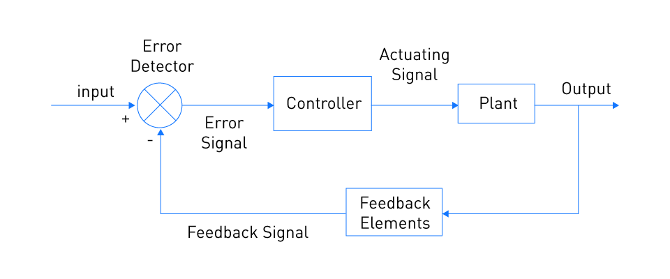
Figure 2: Control system model

Controller Model: The controller is the logic or algorithm that governs the plant's behavior to accomplish desired performance objectives, such as controlling motor speed or preserving a stable output voltage.

• Types of Controllers: Controllers can be either analog (e.g., PID controllers) or digital (e.g., microcontroller-based algorithms). The controller model includes a mathematical representation of these control strategies.

Feedback Loop: Most control systems require a feedback loop, which provides the controller information about the plant's output, which modifies the inputs to maintain the desired performance.

• Modeling Feedback: The feedback loop is modeled in a simulation environment by connecting the plant's output to the controller's input, frequently using sensors that add dynamics such as delays or noise.

Disturbances and Noise: Disturbances are external influences on plant operation, such as electromagnetic interference, load shifts, or temperature fluctuations. Noise is defined as random fluctuations that can disrupt sensor readings or control signals.

• Incorporating Disturbances: Simulation models can incorporate sources of disturbance and noise to assess the control system's robustness. For example, a step change in load might be used to determine how quickly and effectively the controller can recover the desired output.

Steps in Modeling Control Systems

Define System Objectives:

Performance Criteria: Establish the control system's key performance indicators (KPIs), including accuracy, stability margins, and response time. These objectives drive the modeling procedure and assist in determining the performance of different control strategies.

Design Specifications: Define the control system's specifications, such as the operating limits, desired output range, and acceptable error levels.

Develop the Mathematical Model:

Plant Equations: Start by calculating the plant's mathematical model using physical laws such as Newton's laws, Kirchhoff's laws, or thermodynamic principles. This model frequently manifests as a collection of transfer functions or ordinary differential equations (ODEs).

Controller Algorithms: Develop the controller's mathematical representation based on the type of control system. This can incorporate z-transforms and difference equations for digital systems, and Laplace transforms and block diagrams for analog systems.

Implement the Model in Simulation Software:

Simulation Environment: Select the suitable simulation tool based on the system's complexity and requirements. MATLAB/Simulink, for example, is frequently used for modeling analog and digital control systems due to its extensive block libraries and simulation capabilities.

Parameter Initialization: Input the relevant parameters into the simulation environment, including initial conditions, control gains, and component values (resistances, capacitances, and inductances).

Run Simulations and Analyze Results:

Time-Domain Analysis: To assess the performance of the control system, simulate its response over time. The key metrics include rising time, settling time, overshoot, and steady-state error.

Frequency-Domain Analysis: Perform frequency-domain analysis (such as Bode or Nyquist plots) to evaluate the bandwidth and stability of analog control systems.

Parameter Tuning: To achieve the desired performance criteria, modify the control parameters based on the simulation's results. Until the system performs at its best, this iterative process continues.

Challenges in Control System Modeling

Model Accuracy vs. Complexity: A significant challenge in control system modeling is striking a balance between complexity and accuracy. Highly detailed models can make more accurate predictions, but they may demand an extensive amount of computational resources and time. Although simpler models are simpler to simulate, they may miss important dynamicsand produce less reliable results.

Nonlinearities and Discontinuities: Saturation effects, dead zones, and switching operations are examples of nonlinear behavior found in many power electronics systems. For realistic simulations, it is essential to accurately model these nonlinearities, although accomplishing this can be challenging and computationally demanding.

Integration of Analog and Digital Components: In mixed-signal systems, where analog and digital components coexist, maintaining precise interaction between these domains is challenging. Simulation tools must be able to handle continuous and discrete-time signals, as well as the possibility of signal aliasing and quantization errors.

Techniques for Accurate Analog Control System Modeling

In power electronics design, precise modeling of analog control systems is essential to guarantee that the system operates as intended in real-world conditions. Analog control systems rely on continuous signals and are commonly employed in applications that require high-speed response and minimal latency, such as audio amplification, power supplies, motor drives. This section discusses the key techniques for accurately modeling analog control systems, including nonlinearity considerations, component representation, feedback mechanisms.

Component Modeling

Accurate Representation of Passive Components:

Resistors: Resistors are used to establish filter characteristics, time constants, and gain in analog control systems. Real resistors have parasitic effects such as capacitance and inductance, which can impair system performance at high frequencies, whereas ideal resistors are represented as linear components. These parasitics should be accounted for in accurate modeling, particularly in high-frequency applications.

Capacitors and Inductors: In analog control, capacitors and inductors are essential, especially for energy storage and filtering. Accurate models include parasitic resistance (equivalent series resistance) in capacitors and core losses in inductors. To capture their performance in the real world, these components' frequency-dependent behavior needsbe included into precision analog circuits.

Modeling Active Components:

Operational Amplifiers (Op-Amps): Op-amps are frequently employed in analog control systems for feedback control, filtering, and signal amplification. The gain-bandwidth product, slew rate, input bias current, and offset voltage are some of the parameters that should be considered while accurately modeling op-amps. High-precision applications require also consideration for non-idealities including temperature dependency, input noise, and power supply rejection ratio (PSRR).

Transistors: Analog control circuits frequently use field-effect transistors (FETs) and bipolar junction transistors (BJTs). Channel length modulation (CLM) in FETs and the effects of temperature, saturation, and the Early effect in BJTs are examples of nonlinear behavior that should be taken into consideration in accurate transistor models.

Temperature and Environmental Effects:

Thermal Effects: Temperature variations can cause drift in parameters such as resistance, capacitance, and transistor characteristics, which can have significant impacts on the performance of analog components. The process of accurately modeling involves simulating the system's response under various thermal conditions and adding temperature coefficients (the relative change in a physical property due to temperature change) for each component.

Environmental Factors: Analog control systems can also be impacted by environmental factors such as pressure, humidity, and electromagnetic interference (EMI). Although direct modeling is challenging, simulation tools can incorporate environmental disturbances and random noise sources to evaluate the robustness of the system.

Feedback Loop Modeling

Linear vs. Nonlinear Feedback:

Linear Feedback: Linear feedback is utilized in many analog control systems to regulate system output and achieve stable functioning. To model linear feedback, transfer functions or state-space representations are used to characterize the relationship between input and output. To guarantee stability, the frequency response (Bode plots, Nyquist plots) of these systems is frequently modeled and analyzed using tools like MATLAB/Simulink.

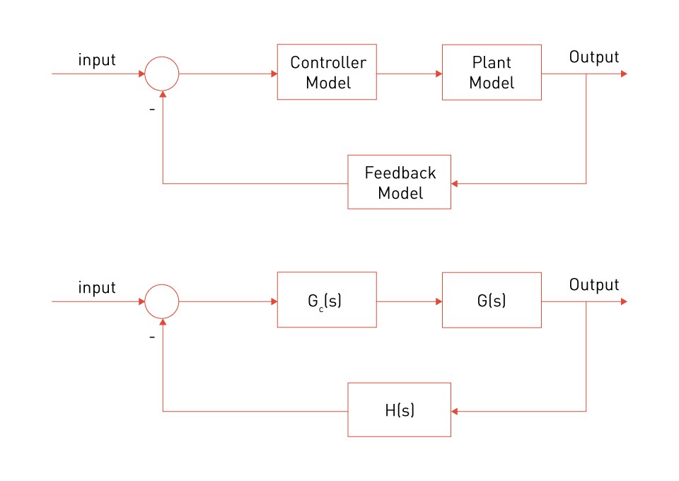
Figure 3: Transfer function-basedmodel of closed loop control system

Nonlinear Feedback: Nonlinear feedback is used in systems when linear control is insufficient, such as oscillators or those with significant signal variations. Accurate modeling of nonlinear feedback necessitates capturing the system's entire dynamic behavior, which is frequently achieved through the use of piecewise linear models (breaking a function into several linear segments) or nonlinear differential equations.

Loop Stability and Compensation:

Stability Analysis: An analog control system's stability is crucial, especially in feedback loops. Techniques such as Nyquist criterion, root locus, and Bode plot analysis can be used to examine stability. To avoid oscillations and guarantee reliable performance, precise modeling of the crossover frequency, phase margin, and loop gain is necessary.

Compensation Techniques: Compensation techniques such as phase-lead compensators, PID tuning, and lead-lag compensation are frequently employed to stabilize an analog feedback loop. Developing comprehensive transfer functions that incorporate the compensator's impact on the dynamics of the overall system is necessary for accurate modeling of these compensators.

Nonlinearity Considerations

Modeling Nonlinear Components:

Diodes and Zener Diodes: Diodes are intrinsically nonlinear components used in rectification, voltage regulation, and protection circuits. To accurately represent diodes, the forward voltage drops, reverse recovery time, and capacitance must be included. Breakdown voltage and dynamic impedance are important considerations for Zener diodes.

Saturation and Clipping: Many analog circuits display saturation or clipping behavior, specifically in op-amps and transistor-based amplifiers. These nonlinear effects, which have the potential to limit the output range or introduce harmonic distortion, should be captured by accurate models.

Time-Varying Nonlinearities:

Hysteresis and Memory Effects: Memory effects can occur in some analog control systems, such as those that use magnetic components or hysteretic controllers. Capturing the hysteresis loop and how it affects the dynamics of the control system is essential for accurate modeling. In power electronics applications such as DC/DC converters with hysteretic control, this is very crucial.

Distortion Analysis: In analog control systems, harmonic distortion is a common issue, especially in applications involving audio or signal processing. To accurately model distortion, simulate the nonlinearities in active components and analyze the ensuing harmonics in the output signal.

Simulation Techniques for Accuracy

Time-Domain Simulation:

Transient Analysis: Time-domain simulation is necessary to analyze the dynamic response of an analog control system to changes in input or operating conditions. Engineers can see how the system responds to step inputs, pulses, or other time-varying signals by using transient analysis in SPICE-based tools such as PSpice. To balance accuracy and computational efficiency, the simulation time step must be adjusted for accurate modeling in the time domain.

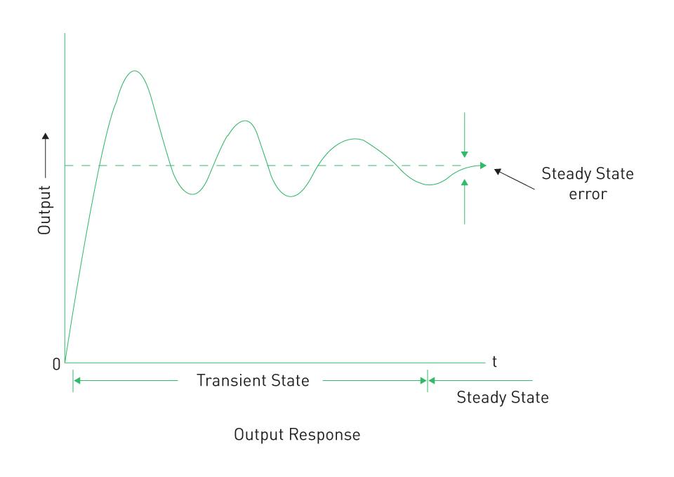
Figure 4: Transient vs. steady-state response

Steady-State Analysis: Steady-state analysis can help assess the long-term behavior of control systems that operate under continuous conditions. This involves performing the simulation until transient effects have subsided and the system has reached equilibrium, at which point performance metrics such as steady-state error and output ripple can be assessed.

Frequency-Domain Simulation:

AC Analysis: When evaluating an analog control system's frequency response, especially its gain and phase margins, frequency-domain analysis is essential. Engineers can design responsive and reliable control loops by using simulation tools that use AC analysis to understand how the system will react to sinusoidal inputs of varying frequencies.

Harmonic Analysis: Harmonic analysis can be used to measure the distortion caused by the control system in applications where nonlinearities are significant. In precision analog applications and audio electronics, where signal fidelity is crucial, this analysis is very important.

Approaches to Digital Control System Simulation

A key component of modern power electronics, digital control systems provide accurate, adaptable, and effective management of electrical systems in a variety of applications. Digital control systems use field-programmable gate arrays (FPGAs), digital signal processors (DSPs), or microcontrollers to implement digital control algorithms. In contrast to analog control systems, which operate on continuous signals, digital control systems process discrete signals. Before implementing hardware, digital control systems must be accurately simulated to predict system behavior, maximize performance, and guarantee reliability. The primary techniques for modeling digital control systems are explored in this section, with a focus on the significance of discretization, time-step selection, and digital controller modeling.

Discretization of Continuous-Time Models

Discretization:

Digital control systems require discretization, which is the process of converting continuous-time models into discrete-time models. In digital control, signals are sampled at specific intervals, and calculations are made using the sampled values instead of continuous signals.

Sampling Rate: In digital control system simulation, selecting the appropriate sample rate is crucial. It must be low enough to prevent an excessive computational burden and high enough to capture the system's essential dynamics without causing aliasing. A theoretical foundation is provided by the Nyquist-Shannon sampling theorem, which states that the sample rate ought to be at least twice the bandwidth of the signal.

Where f_B is the signal bandwidth and f_S is the sampling frequency.

Techniques for Discretization:

Zero-Order Hold (ZOH): ZOH is a popular discretization technique that maintains the control signal consistent during sampling periods. Although this method is simple and quick to use, systems with fast dynamics may have delays or inaccuracies.

First-Order Hold (FOH): FOH provides a better approximation of the continuous signal than ZOH, especially in systems with higher-frequency components, because it interpolates linearly between sampled values.

Tustin (Bilinear) Approximation: Tustin's method uses the z-domain to approximate the s-domain in order to map continuous-time transfer functions to discrete-time. Because it maintains accuracy and stability, this method is frequently employed, particularly in feedback control systems.

Modeling Digital Controllers

Digital Control Algorithms:

Proportional-Integral-Derivative (PID) Controllers: In digital control systems, PID controllers are among the most widely used. The emulation approach to digital controller design consists of two steps: first, build a continuous controller, in this example a PID, and then discretize using methods such as the trapezoidal rule, forward Euler, or backward Euler. The controller's performance, especially its responsiveness and stability, is impacted by the method selection. This method is preferred when fast sampling is possible.

State-Space Models: State-space representations can be used to simulate digital controllers for complex systems. With this method, the continuous-time state-space equations are discretized, usually using zero-order hold techniques or matrix exponential methods.

Implementation in Simulation Tools:

MATLAB/Simulink: A flexible framework for modeling digital controllers is offered by MATLAB/Simulink. The software comes with pre-built blocks for digital filters, PID controllers, and custom code implementations. By establishing the sample rate, using various discretization techniques, and evaluating the system's reaction to diverse inputs, engineers can model the controller's performance.

Hardware-in-the-Loop (HIL) Simulation: HIL simulation provides a method to evaluate digital controllers for real-time digital control systems in a virtual environment that mimics physical hardware. When it comes to safety-critical applications like automotive or aerospace systems, this method is very helpful for verifying control algorithms prior to deployment.

Time-Step Selection in Digital Simulations

Choosing the Appropriate Time Step:

Fixed vs. Variable Time Steps: The choice between fixed and variable time steps has a significant impact on the computing efficiency and simulation accuracy of digital control systems. Numerous design- and application-specific considerations, such as frequency bandwidth, required simulation accuracy, and network complexity, influence the time step selection. Another consideration is the inverse relationship between time step and simulation run time. Although fixed time steps are easier to build and frequently employed in real-time simulations, accurate capture of fast dynamics may necessitate a lower step size. On the other hand, variable time steps offer a balance between simulation speed and accuracy by dynamically adjusting according to the behavior of the system.

Impact on Stability: The digital control system's stability is directly impacted by the time step. A time step that is too large may cause numerical instability, in which case the simulated system might exhibit irrational behavior such as divergence or oscillations. On the other hand, a small-time step raises the computing strain without necessarily increasing accuracy in proportion.

Best Practices:

Start with Theoretical Analysis: To estimate an appropriate time step, start by examining the dynamics of the control system. This can be done by looking at the system's highest frequency component or dominant time constant.

Iterative Refinement: Iteratively modify the time step during the simulation in response to performance observations, focusing on crucial aspects including overshoot, settling time, and rise time.

Real-Time Constraints: The time step for real-time digital control systems needs to match the processing power of the hardware so that the control algorithm can execute within the allotted time without missing deadlines.

Modeling Quantization Effects and Delays

Quantization in Digital Control Systems:

In digital control systems, quantization is the process of mapping continuous signal values to discrete levels. It also creates quantization noise, which can affect system performance, especially in high-precision applications.

Modeling Quantization: Simulation tools can simulate quantization effects by including quantization blocks or functions that imitate the behavior of digital-to-analog converters (DACs) and analog-to-digital converters (ADCs). This enables engineers to evaluate the effects of quantization on system stability, control accuracy, and signal fidelity.

Modeling Delays:

Sources of Delays: A number of factors, including communication latencies, actuator response times, and computational/processing delays, can cause delays in digital control systems. If these delays are not appropriately considered, system performance can deteriorate or even lead to instability.

Incorporating Delays into Models: To model these impacts, simulation tools include delay blocks that can be added to the control loop. Engineers can experiment with different delay values to see how they affect the system's stability and modify the control algorithm accordingly to prevent adverse effects.

Testing and Validation of Digital Control Systems

Simulating Real-World Conditions:

Robustness Testing: Digital control systems should be evaluated under a range of operating conditions, including extreme situations such as abrupt load changes, sensor noise, and component failures, in addition to standard simulations. Robustness testing is facilitated by simulation tools such as MATLAB/Simulink, which allow fault injection, parameter sweeps, and Monte Carlo simulations.

Validation Against Physical Models: The digital control system must be validated against physical models or prototypes for critical applications. A strong tool for this is HIL simulation, which gives the digital controller real-time interaction with a physical plant model and a high degree of assurance over the system's performance prior to deployment.

Iterative Design and Optimization:

Continuous Refinement: Digital control system design is frequently an iterative process in which the design of algorithms, system architecture, and control parameters are optimized based on simulation results. Frequent simulation at the design stage lowers the chance of expensive redesigns later in the development cycle by assisting in the early identification and correction of issues.

Feedback from Testing: The digital control system can be continuously improved to meet all performance, reliability, and safety requirements by incorporating feedback from physical testing and validation into the simulation model.

Hybrid Modeling for Mixed Signal Systems

Modern power electronics and control applications frequently use mixed signal systems, which blend analog and digital components. These systems leverage the advantages of digital circuits' flexibility, accuracy, and programmability as well as analog circuits' high-speed operation and continuous signal processing. In order to accurately simulate the interactions between these two domains and guarantee that the system operates reliably in real-world scenarios, hybrid modeling is crucial. This section explores the principles and techniques of hybrid modeling for mixed signal systems, with a focus on the integration of analog and digital components in simulation environments.

The Need for Hybrid Modeling

Complexity of Mixed Signal Systems:

Integration Challenges: Mixed signal systems can include tightly coupled analog and digital circuits including analog-to-digital converters (ADCs), digital-to-analog converters (DACs), power amplifiers, and digital controllers. In order to effectively forecast real-world behavior, simulations must accurately capture the complexities introduced by the interaction of these components, which can include noise, signal distortion, and timing issues.

Applications in Power Electronics: Hybrid modeling is especially crucial for applications such as power management, where digital systems (including microcontrollers and DSPs) govern analog power stages (such as converters and inverters). Robust performance, steady control, and effective power conversion are guaranteed in these applications by accurate modeling.

Benefits of Hybrid Modeling:

Comprehensive Simulation: Engineers can simulate the full system behavior and capture the complex interactions between domains by modeling both analog and digital components together. This comprehensive approach eliminates the possibility of design errors that could occur if each domain was simulated individually.

Early Detection of Issues: Engineers can use hybrid models to uncover potential issues such as signal integrity problems, timing mismatches, and EMI susceptibility early in the design phase, before committing to hardware prototyping.

Techniques for Hybrid Modeling

Co-Simulation:

Co-simulation is the process of simulating a system by employing several simulation engines or tools designed for the analog and digital domains, either simultaneously or sequentially. By exchanging data at predefined interfaces, the simulators guarantee accurate modeling of both analog and digital components.

Tools and Environments: MATLAB/Simulink is frequently used for co-simulation, in which the analog circuit is modeled using tools like SPICE or Simscape, while the digital control system is modeled by Simulink. Using Verilog-AMS or VHDL-AMS, which are hardware description languages that facilitate mixed-signal modeling, is an additional strategy.

Discrete Event and Continuous Time Modeling:

Discrete Event Modeling for Digital Systems: Digital components are commonly modeled as discrete event systems, in which the occurrence of specific events (such as clock edges or logic state changes) causes the system's state to change at discrete time intervals. Digital controllers, logic gates, and communication protocols can all be effectively modeled using this method.

Continuous Time Modeling for Analog Systems: Analog components are modeled as continuous time systems, in which differential equations control the system's state as it changes continuously over time. Analog filters, amplifiers, and power converters are modeled using this method.

Coupling Discrete and Continuous Models: Accurately coupling the digital models for discrete events with the analog models for continuous time is essential in hybrid modeling. To match the timing of signals, this entails carefully controlling the data exchange between the two domains, frequently utilizing interpolation and extrapolation techniques.

Handling Signal Conversions:

Analog-to-Digital Conversion (ADC) Modeling: Continuous analog signals are converted into discrete digital values using ADCs. Accurate modeling of ADCs requires capturing issues such as sampling rate limitations, quantization noise, and input bandwidth. The fidelity of the digital representation of the analog signal can be significantly impacted by these factors.

Digital-to-Analog Conversion (DAC) Modeling: DACs convert digital signals back to continuous analog signals. Accurate DAC modeling considers the reconstruction filters, conversion resolution, and potential error sources including voltage reference stability and clock jitter.

Managing Timing and Synchronization:

Clock Domain Crossing: In mixed signal systems, digital components frequently operate at different clock rates than analog components. To avoid timing errors or data corruption, it is essential to make sure that these clock domains are properly synchronized. To handle these challenges in simulation, methods including clock domain crossing (CDC) checks and metastability analysis are employed.

Timing Delays and Latencies: Delays are unavoidable in digital systems because of data buffering, signal propagation, and processing. To guarantee that the analog components can respond to the digital control signals in an appropriate manner, these delays must be precisely modeled. Delay blocks or models are commonly used in simulation tools to account for these effects.

Simulation Tools for Hybrid Modeling

Integrated Simulation Environments:

MATLAB/Simulink with Simscape: MATLAB/Simulink, when combined with Simscape, creates a powerful environment for hybrid modeling. Simulink manages the digital control logic, while Simscape enables the physical modeling of analog components. Co-simulation on a single platform is made possible by the two being seamlessly integrated.

Cadence and Synopsys Tools: Tools such as Cadence Virtuoso and Synopsys Saber provide extensive co-simulation environments for more complex mixed signal design. With great accuracy and detail, these tools facilitate the integration of digital models described in Verilog or VHDL with SPICE models for analog circuits.

Multi-Domain Modeling Languages:

VHDL-AMS and Verilog-AMS: The purpose of these hardware description languages is to model mixed signal systems. They enable smooth simulation and synthesis by enabling the simultaneous description of analog and digital behavior within the same model.

PSpice for TI and Mixed Signal Extensions: An expansion of the traditional PSpice environment, PSpice for TI facilitates mixed-signal simulation by integrating digital models and allowing co-simulation with analog circuits. This tool is especially useful for power electronics applications, which frequently involve mixed signal interactions.

Hardware-in-the-Loop (HIL) for Mixed Signal Systems:

Real-Time Simulation: HIL systems enable the real-time simulation of mixed signal systems, in which the analog/real-world plant is simulated in real-time while the digital controller is implemented in hardware (such as an FPGA or microcontroller). This method is extremely useful for testing mixed signal designs under realistic operating conditions.

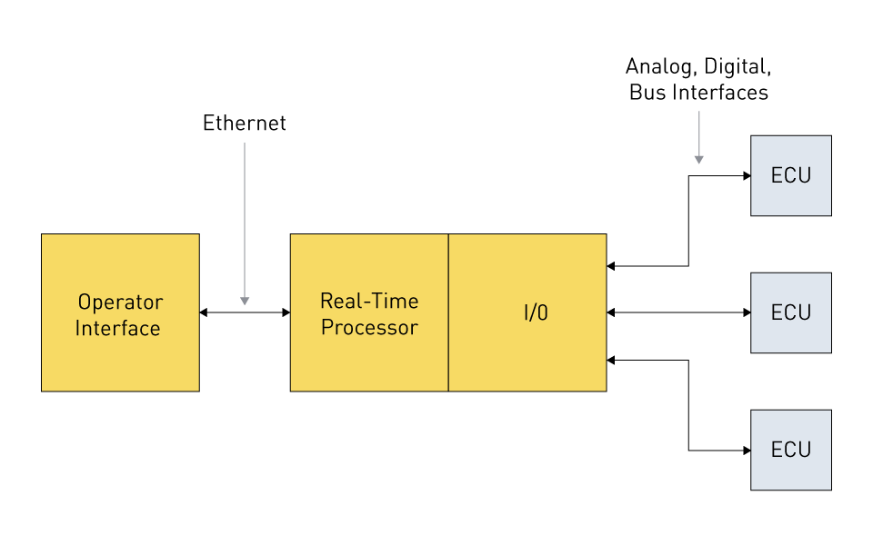
Figure 5: HIL testing of multiple-ECU systems such as airplanes, automobiles, etc.

Interaction with Physical Components: The digital controller in HIL setups can interact with both real-world sensors or actuators and simulated analog components, offering a high level of realism and facilitating extensive testing prior to full system integration.

Challenges and Solutions in Hybrid Modeling

Signal Integrity Issues:

Noise and Crosstalk: Systems with mixed signals are prone to crosstalk between the digital and analog domains and noise. Accurate modeling necessitates capturing these effects and assessing their impact on signal integrity. To overcome these challenges, simulation tools frequently offer the option to simulate signal coupling and noise sources.

Power Supply Interactions: In mixed signal systems, the shared power supply can result in interactions such as supply noise or voltage drops that impair performance. Hybrid models should incorporate power supply models that account for these effects, especially in low-power or high-precision applications.

Computational Complexity:

Simulation Speed vs. Accuracy: Hybrid models can be computationally demanding, particularly when simulating accurate analog behavior alongside complex digital logic. A significant challenge is striking a balance between simulation speed and accuracy, which frequently calls for simplifications or the usage of behavioral models for less important components.

Model Abstraction: Engineers may employ hierarchical modeling to manage complexity, which uses simplified or abstract models for less important system components and detailed models for essential components. This method preserves overall accuracy while reducing simulation time.

Validation and Verification:

Model Verification: It is crucial to ensure that the hybrid model adequately represents the real system. This involves employing techniques including formal verification, simulation-based testing, and comparison with actual data to confirm that the model's behavior matches expected results under various operating conditions.

Model Calibration: Accuracy can be improved by calibrating the hybrid model using measured data from prototypes or earlier designs. By modifying model parameters to more closely match real-world behavior, this procedure ensures that simulation results accurately reflect system performance in the real world.