Field-Oriented Control for PMSMs Utilizing a Dynamic Speed Observer
By Jia Li, Engineer, Monolithic Power Systems
Permanent magnet synchronous motors (PMSMs) are prevalently used in industrial manufacturing for electric vehicles, electric airplanes, robotics, household electric appliances, and more. Vector control is normally implemented to drive permanent magnet synchronous motors (PMSMs) to have better dynamic response and to use the full machine potential.
Determining the rotor speed and position is mandatory to achieve vector control. Optical quadratic sensors and Hall-effect sensors are the most commonly used to measure the speed and position of the motor. However, optical quadratic sensors and Hall-effect sensors are expensive, increasing drive cost.
One promising solution for the PMSM drive is a combination, using a low-cost magnetic angular sensor and a dynamic observer to estimate the accurate rotor speed. The MPS motor control module presented in this article includes a motor control ASIC, a magnetic angular sensor, three-phase MOSFET power stage, and pre-drivers on one PCB to fit NEMA 23 and NEMA 17 format motors.
The motor control ASIC provides excellent computation ability for applications such as electrical motor drives. It works with the MA702, a 12-bit resolution magnetic angular sensor that detects the absolute position of the PMSM rotor. The MA702 is less costly than optical quadratic sensors and Hall-effect sensors. Knowing the rotor position throughout the entire process enables the motor speed to be detected by building a dynamic state observer based on the PMSM’s mechanical equation. The ASIC uses the dynamic observer to filter out the position measurement noise and estimate the rotor speed to employ field-oriented control (FOC) for the PMSM.
FIELD-ORIENTED PMSM CONTROL
Three-phase PMSM machine equations can be expressed with Equation Set (1):
(1)
$$v_{as}=r_s i_{as}+ρλ_{as}$$
$$v_{bs}=r_s i_{bs}+ρλ_{bs}$$
$$v_{cs}=r_s i_{cs}+ρλ_{cs}$$
$$T_e = {P\over 2} λ'_ m [cos (θ_e) i_{as} + cos (θ_e - {2\over 3} π ) i_{bs} + cos (θ_e + {2\over 3} π) i_{cs}] $$
Where v, i, and λ are the voltage, current, and flux, respectively. The subscripts a, b, and c represent the variables in phases a, b, and c. Subscript s is the stator variable, ρ represents the derivative of the certain value, and P is the number of poles of the PMSM.
The electromagnetic torque $T_e$ is produced by the three-phase current and the rotor flux. $λ'_m$ is the rotor flux sensed on the stator side of the PMSM. The angle $θ_e$ is the electrical angle between the rotor flux and the stator a phase.
To achieve FOC for PMSM, a dynamic model under q-d is required to decouple the air gap-flux and electromagnetic torque. Following the Clarke-Park transformation, the PMSM model in Equation Set (1) under the synchronous rotating q-d frame is calculated with Equation Set (2):
(2)
$$v_{qs}=r_s+ω_r λ_{ds}+ρλ_{qs}$$$$v_{ds}=r_s-ω_r λ_{qs}+ρλ_{ds}$$$$λ_{qs}=L_s i_{qs}+L_m i_{qr}$$ $$λ_ds=L_s i_{ds}+L_m i_{dr}$$
Where the subscripts q-d are the q-d axis variables. $L_s$ is the self-inductance and $L_m$ is the mutual inductance of the machine. To further simplify the control, the rotor flux should be aligned on the d-axis while there is zero rotor flux on the q-axis. The flux is calculated with Equation Set (3):
(3)
$$λ_{qs}=L_s i_{qs}$$
$$λ_{ds}=L_s i_{ds}+λ'_m$$
The electromagnetic torque is estimated with Equation (4):
(4)
$$T_e = {3\over 2} {P\over 2} (λ'_m i_{qs} + (L_d - L_q) i_{ds}i_{qs}$$
Following the transformation steps from Equation Set (1), Equation Set (2), Equation Set (3), and Equation (4), the magnetic flux can be directly controlled by the d-axis current. With a constant $i_ds$ , the torque $T_e$ can be controlled directly by manipulating the q-axis current. If keeping $i_ds=0$, then the electromagnetic torque is directly proportional to $i_qs$.
Figure 1 shows the PMSM FOC schematic, obtained from the derivations above.

Figure 1: PMSM FOC Schematic
The outer loop reference compares to the measured variables, and feeds the error to a controller (PI controller being the most commonly used) to generate the command torque current $IQ_{ref}$. The d-axis current reference $ID_{ref}$ is set according to the magnetic flux requirement. The output of the current regulators/controllers $VD_{ref}$, $VQ_{ref}$, $VD_{ref}$, and $VQ_{ref}$ are the input for the space vector PWM (SVPWM). The SVPWM block generates the gate signals for the inverter to drive the PMSM.
DYNAMIC OBSERVER BASED SPEED-SENSORLESS DRIVE
The MA702 detects the position of a permanent magnet $θ_e$. The speed of the rotor can be calculated as $ω_e=ρθ_e$. As a digital sensor, the MA702 inevitably introduces noise into the measured position. If taking the motor speed directly by using the position differential, the control scheme will be deteriorated. Adding a digital filter/estimator to the system is a natural solution to this problem.
The system estimator can be built based on the mechanical PMSM model using Equation Set (5):
(5)
$$ρω_m=- {B\over J} ω_m- {T_l\over J} + {T_e\over J}$$
$$ρθ_m=ω_m$$
Where $T_e$ is the electromagnetic torque and $T_l$ is the load torque. $ω_m$ and $θ_m$ are the mechanical rotor speed and position, compared to the electrical rotor speed and position $ω_e$ and $θ_e$. The mechanical speed and position times ${P\over 2}$ is equal to the electrical speed and potions. P is the pole number of the PMSM. The parameters J and B represent the PMSM inertia and the combined viscous friction of rotor and load, respectively.
The MA702 feeds the absolute rotor position to the motor control ASIC, making the mechanical model system matrix A a simple 3x3 matrix with only two non-zero elements. A simpler system matrix helps decrease the computation burden on the MCU, making the algorithm easier to implement and faster to execute.
Discretize the mechanical model of the PMSM in Equation Set (5) using Euler’s method. The state variables x, ∈, and $R^n$ are the states of a system process that can be expressed in discrete time with Equation Set (6):
(6)
$$x_k=Ax_{k-1}+Bu_{k-1}+w_{k-1}$$$$y_k=Hx_k+v_k$$$$p(w) \sim N(0,Q)$$$$p(v) \sim N(0,R)$$
Where u is the input variable and y is the output measurement. w and v are the process and measurement noise with noise covariance of Q and R, respectively.
Following classic control theory, a state estimator with estimator gain K can be calculated with Equation (7):
(7)
$$x ̂_{k|k}=x ̂_{k|k-1}+K(y_k-Hx ̂_{k|k-1})$$
The notation $a_{n|m}$ represents the estimation of a at step n is up to the observation of step and $m\le n$. The carat (^) denotes that the variable is estimated. Unlike the classic state observer using a constant gain K, a dynamic observer recursively updates its estimator gain K with each iteration.
Compared to the FOC schematic (see Figure 1), the dynamic speed observer based drive schematic uses machine measurements as the system input to execute the observer (see Figure 2). The dynamic observer outputs the filtered/estimated rotor speed. The rotor position is used to conduct the FOC of the PMSM.

Figure 2: Dynamic Observer Based PMSM FOC
SIMULATION RESULTS
Matlab/Simulink is used to carried out the simulation results. The motor used to validate the algorithm is MPS eMotion SystemTM smart motor MMP757094-36. The MMP757094-36 is part of a family of fully integrated smart motor solutions for servo motor applications. Table 1 shows the motor parameter.
Table 1: Motor Parameter
|
Stator phase resistance |
600mΩ |
|
Stator phase inductance |
600µH |
|
Motor inertia |
210g * cm2 |
|
Torque constant |
76mN * m/A |
|
Pole pairs |
4 |
Figure 3 shows how the estimated speed traces the actual motor speed. The estimated and the actual speed both go to steady state after about 0.05s. Figure 4 shows that the absolute value of the matrix determinant of the error covariance drops to zero after the speed response stabilizes. The dynamic observer gain changes with the speed response. After the transient period, the observer gain K becomes a constant gain.

Figure 3: Speed Response
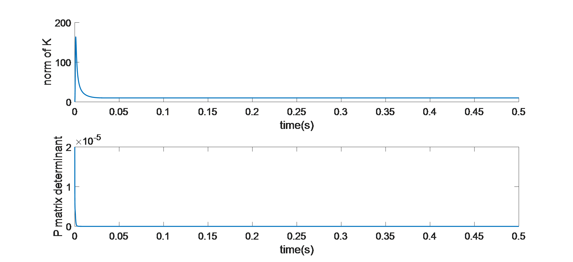
Figure 4: Error Covariance and Observer Gain Dynamics
REAL-TIME HARDWARE RESULTS
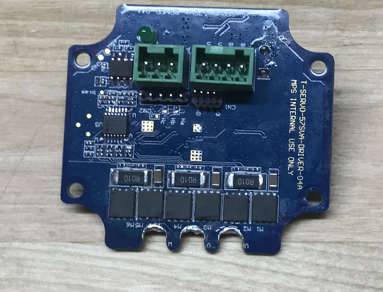
To validate the algorithm, real-time hardware experimental results were also measured. The motor control module, designed for NEMA 23 57mm motors, can be directly mounted on the motor.
 |
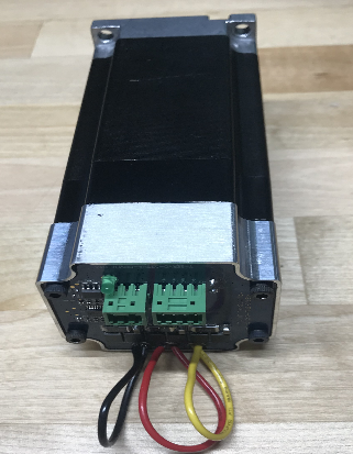 |
Figure 5: MPS Motor Control Module (Left) and MPS Smart Motor (Right)
As discussed in the previous section, having the MA702 angular sensor feeding the absolute rotor position to the motor control ASIC makes the implementation of the dynamic observer recursive iteration easier and less of a computation burden. Since the measurement is only one variable, instead of going through a complicated matrix transformation, the observer gain calculation becomes simple division. The entire dynamic observer calculation takes less than 20µs for each iteration.
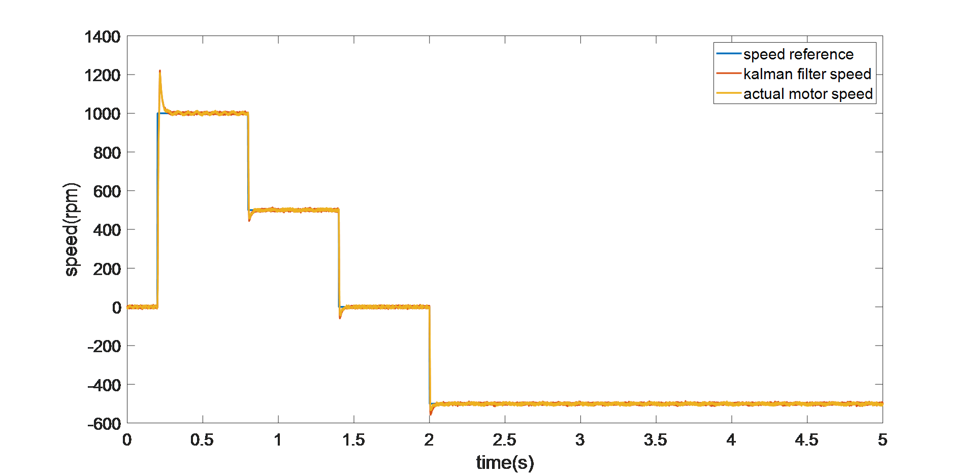
Figure 6: Step-Speed Response in Real-Time
Figure 6 shows that a wide range of speed references, from 1000rpm to -500rpm, are fed to the simulation system with step changes. The dynamic observer estimated speed can still track the motor speed facing different speed reference steps. The algorithm can also give a stand-still reference.
CONCLUSION
This article presents a promising solution for PMSM FOC as a combination of a low-cost magnetic angular sensor and a dynamic observer to estimate the accurate rotor speed. The algorithm is implemented in the motor control ASIC from MPS. The MA702 provides a high-resolution, on-board angular sensor, so the algorithm avoids the high-dimension matrix inverse calculation. This eases code development and time spent on calculation. Both the simulation and real-time validation results show the proposed solution has good dynamic performance and is able to control the PMSM given different speed references.
_________________________________
Did you find this interesting? Get valuable resources straight to your inbox - sent out once per month!
Technical Forum
 Latest activity 6 days ago
 2 Comments
Latest activity a week ago
2 Comments
Latest activity 4 weeks ago
1 Comment
2 Comments
Latest activity a week ago
2 Comments
Latest activity 4 weeks ago
1 Comment
Log in to your account
Create New Account